Understanding SPP Statistical Forecasting and the DRP Matrix
Executive Summary
- We cover how forecasting works in SAP SPP, explaining the forecasting models, dealing with declining demand.
- We take you through the SPP forecasting screens.

Introduction to SPP Statistical Forecasting
Forecasting includes the whole life cycle of a product, from phase-in planning for new products via various product interchangeability types to phase out planning.
How Forecasting Works in SPP
SPP has some forecasting models. This includes the following:
- Exponential Smoothing
- Regression (in this case, it is not causal but uses least squares on the demand history to develop the future trend line)
- Declining Demand Forecast
- Various Moving Average
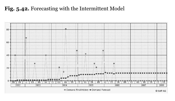
- Intermittent (specialized for service parts)
- Seasonal (seasonal coefficients must be determined at IMG: APO –> Supply Chain Planning –> SPP –> Forecasting –> Define Seasonal Coefficients

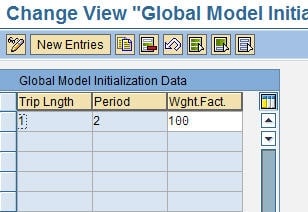
You can see the coefficient was set up for one period. There are 12 periods for which the indices can be set up (for months).
These coefficients are then assigned to the forecast profile. Seasonal coefficients are assigned to the Model Parameter tab in the DRP Matrix.
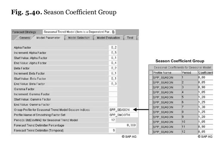 As with Demand Works Smoothie, at least 24 months are required to use the seasonal model. If 36 months of demand history is available, the trend is calculated as the three years’ weighted average. The annual weighting factors are defined in the forecast profile.
The intermittent model derives the Croston’s, which is not anything much more than a long moving average.
Declining Demand
This is used for forecasting at the end of a service part’s life cycle. The product must not be marked as a “new product,” and forecasts must exist for the current period.
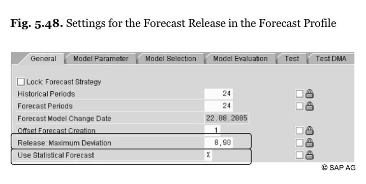
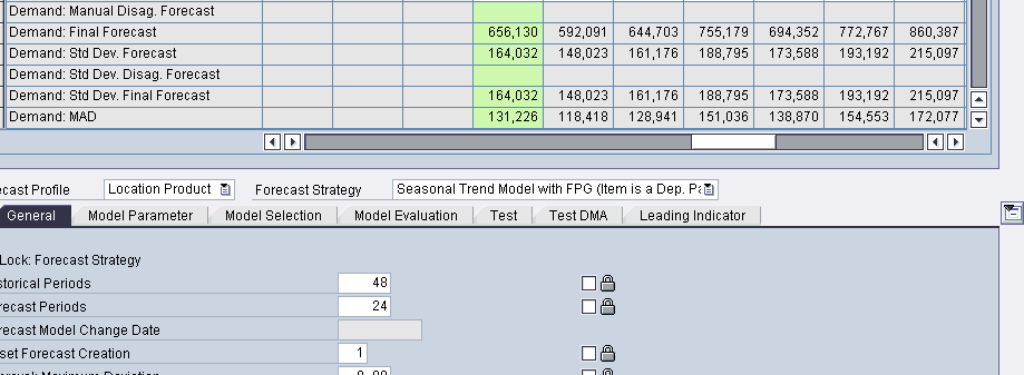
Standard deviation is displayed in the forecasting planning book. Standard deviation is calculated together with the MAD after performing the forecast. The standard deviation for future periods is required for the calculation of the EOQ and the safety stock.
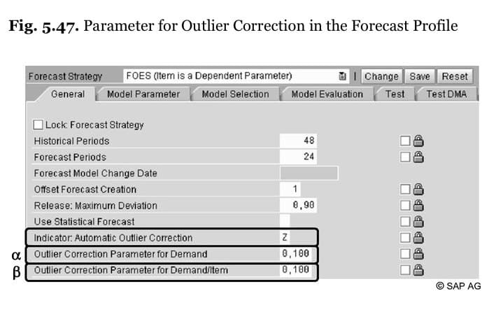
Outliers
Outlier control is on the General tab.
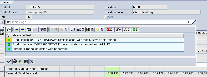
 As is the forecast approval
 Here is the forecast approval screen.
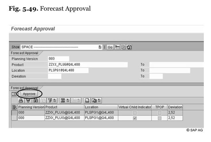 The forecast approval orders are created and displayed in the product view with the transaction /SAPOAPO/RRP3. DRP requires these forecast orders. Before the forecast, approval of the forecast only exists in the time series in the TSDM.
The forecast must be initialized at the following path:
IMG: APO –> Supply Chain Planning –> SPP –> Forecast –> Initialized Base Values
 Forecasting Screens
In the DRP Matrix (an identical layout exists for Interactive Planning), we can see the graph’s forecasting. Think of this as a more detailed view of a planning book, but much easier to use. However, just as importantly, the DRP Matrix contains an enormous number of settings that control the forecast.
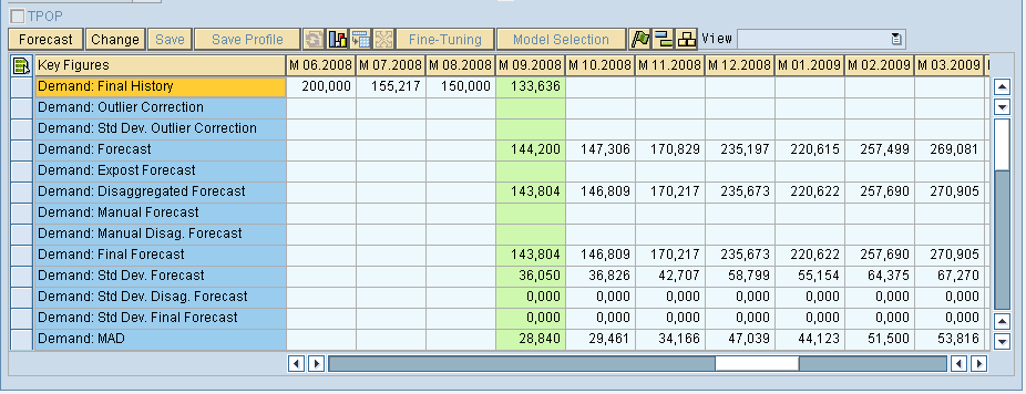
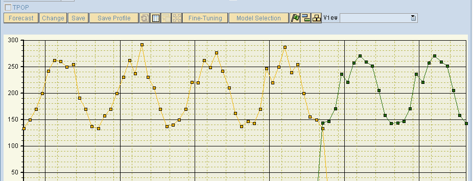
 Here we have two line items selected, and we ask the system to draw a graph. This allows us to compare history to the forecast.
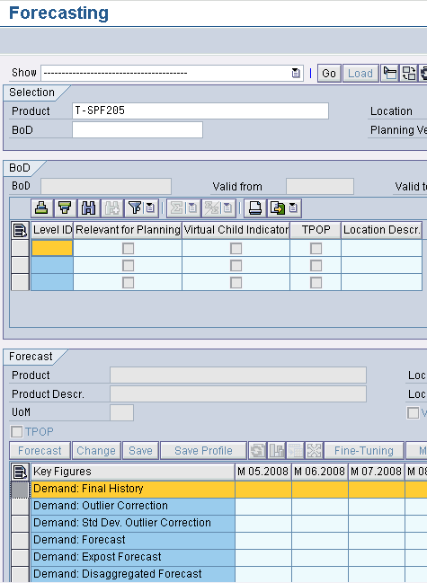 Now, this shows the bill of distribution.
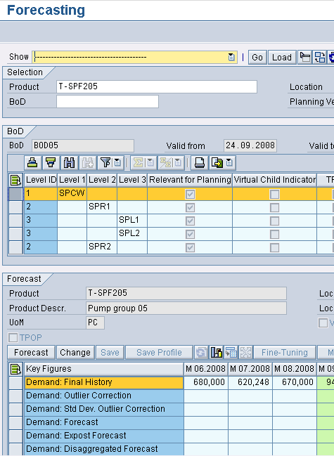 Here we can see the trend line in the DRP Matrix. The DRP Matrix only works for one product and does not support aggregation as the planning book does. However, although it lacks aggregation, it is from a usability perspective as a far superior tool.
 <br ” />Now that we have seen the controls on the forecast, we will navigate to the planning service manager. Under the parameters tab, all types of controls, such as Alpha, Beta, and Gamma (smoothing factors).
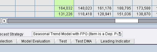
As you can see, the Seasonal Model with Fixed Periods is the default model.
DP also has seasonal forecasting capability. Learn more about it; see this article.
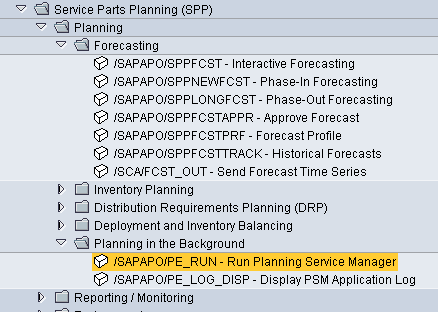
Next, we want to run the planning service manager or PSM. This allows us to access functionality that is distributed through SCM. It is a new concept to SCM and should be well understood.
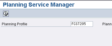 The planning service manager is an essential part of SPP.