
How to Best Use Aggregate Supply Planning in SAP APO
Executive Summary
- Most aggregated planning is performed in demand planning. However, aggregated planning can be used for supply in APO and other systems.
- Aggregated supply planning in APO can be performed when the supply planning load is calculated outside of the system.

Introduction to Aggregate Supply Planning
Aggregated planning is for supply is one of the more advanced types of planning or planning overlays. You will learn how aggregate supply planning works and how it is configured in APO.
What is Aggregate Supply Planning?
Aggregate supply planning is the aggregation of planning by a supply element. Aggregate supply planning can be performed by product, by location, or by time.
Background on Aggregate Supply Planning
Supply planning primarily deals at the product location. Forecasting applications, such as SAP DP, will often perform a variety of aggregations. Understanding how to aggregate is one of the significant challenges to effective forecasting. And many companies cannot aggregate the way they would like because, in my opinion, is some limitations on aggregation and disaggregation vis-à-vis other demand planning applications that I have used, which is covered in the article.
With all of this different type of aggregation that occurs in demand planning, it is, of course, necessary to associate the level of aggregation in DP to the level of aggregation required by SNP when the forecast is released to supply planning.
Any aggregation can be performed in demand planning that can help improve the forecast. Demand planning can aggregate per product, location, or time dimensions. However, at some point, when the demand plan is released to supply planning, it must be disaggregated to a product location combination. It must be placed into the planning buckets that are used by supply planning.
This disaggregation must occur in the way required by supply planning because, as shown above, supply planning applies both supply planning methods and method modifiers based on a product location.
A lack of consideration for how the forecast will be used by supply planning is partially to blame for activities, which are taken up in demand planning that benefit neither the supply planning nor the company. I call this inwardly focused demand planning and have presented on this topic. This article covers making demand planning “friendly” to supply planning, which means engaging in activities that benefit supply planning and looking at supply planning as a customer of the demand planning output.
Aggregation in Demand Planning Versus Aggregate Supply Planning
Supply planning is primarily about applying supply planning methods and method modifiers at the product location combination, or what is also referred to as the product location database.
The existence of a product location master allows each product location to be managed differently regarding both the procedure that is applied to the product location. For more details, see my book Multi-Method Supply Planning in SAP APO and the parameters and method modifiers that control the planning for the product location.
This is an important consideration, which is sometimes lost on demand planning. In the vast majority of cases, no matter what type of aggregation is performed in demand planning, the forecast must eventually be broken down into the product location to be used by supply planning. Therefore, a disaggregation procedure must occur in any demand planning system to get the forecasting results in a usable form by supply planning.
Demand Planning Versus Supply Planning
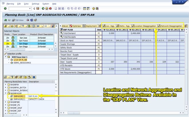
Therefore while demand planning has unlimited flexibility in how it aggregates along the time, location, and product dimensions, supply planning is performed at a product location combination. Now there is a caveat to this, which is the fact that there is aggregation functionality in SNP. However, it is essential to note that the aggregation feature is very rarely implemented in SNP. I have seen one instance of aggregation in SNP placed into production, and it was location aggregation. SNP can aggregate the plan based upon the following dimensions.
- Product
- Resource
- Location
The functionality of aggregation in demand planning is different from the functionality in supply planning. Aggregation in SNP works much differently than does in DP. For instance, while hierarchies and attributes are built right into the Data Workbench in DP and every DP implementation, I am aware of using a hierarchy and most often uses attributes. There are six different types of aggregation available within SAP SNP. One of the six types – the Location Product, is a derivative of two other types of aggregation, the Product and the Location that are then auto-generated from these two hierarchies.
Hierarchy Types
These hierarchy types are listed below:
- Product
- Location
- Location Product
- Resource
- PPM/PDS
- Transportation Zone
All of the hierarchies are created similarly, except for one, which is the location product hierarchy. Auto-generating pre-existing location and product hierarchies create this hierarchy.
Aggregation in Demand Works Smoothie
One idea behind aggregation in demand planning software is that aggregation can improve the visibility and insight into the forecasting data. For those who have used effective demand planning software, which has aggregation capabilities, this is truly advantageous.

Demand Works Smoothie is one of the better aggregation/attribute-based forecasting systems that I have used. One can see in the screenshot above that I am currently at the Half Pint level in the hierarchy, which begins at City/Location Description (Los Angeles, San Diego, San Francisco, San Jose). It then moves to the type Ice Cream Type (Extra Rich or Normal) and then the Flavor (Chocolate, Cookie Dough, Vanilla) and finally Size (Half Pint, Pint)
A second reason for performing aggregation is reporting out to various interested parties how much is forecasted to be sold by a particular category (which is an aggregation). The third reason for aggregation in demand planning is using top-down forecasting to improve the forecast. This creates a forecast for a grouping of products and eventually disaggregates down to the SKU based upon disaggregation/allocation logic (which can be adjusted in some applications). Forecasts based upon aggregations tend to be more accurate, demonstrate seasonality and trends more clearly, and possess less bias. Different groups of products or channels will be optimally forecasted at different aggregation levels and or using different hierarchies.
Aggregate Demand Planning Versus Aggregate Supply Planning
The idea behind aggregate supply planning is a bit different from demand planning. With supply planning aggregation, the concept is that a load can be applied to the parent entity (product, resource, location), which is then disaggregated to the child entities (product, resource, location). The benefit is that the load is more equally shared and thus more efficiently shared. It can also be valuable when the load is calculated outside of the system. An excellent example of this is when a company’s capacities for resources are calculated as a group during a rough cut capacity planning process. If a company needs to allocate this load in an aggregated manner, aggregate planning is supposedly used. (Those interested in resource aggregation can see the following links for
With aggregate supply planning, the concept is that a load can be applied to the parent entity (product, resource, location), which is then disaggregated to the child entities (product, resource, location). The benefit is that the load is more equally shared and thus more efficiently shared. It can also be valuable when the load is calculated outside of the system. A good example of this is when a company’s capacities for resources are calculated as a group during a rough cut capacity planning process. If a company needs to allocate this load in an aggregated manner, aggregate planning is supposedly used. (Those interested in resource aggregation can see the following links for
When the Load is Calculated Outside of the System
It can also be valuable when the load is calculated outside of the system. A good example of this is when a company’s capacities for resources are calculated as a group during a rough cut capacity planning process. If a company needs to allocate this load in an aggregated manner, aggregate planning is supposedly used. (Those interested in resource aggregation can see the following links for here and here)
After reviewing how to aggregate supply location aggregation works and seeing it demonstrated as well as discussing the issue in great depth with a previous client, I can say that at most, it can plan redeployments within a single echelon (an echelon being a level of locations in the supply network – such as distribution centers, or regional distribution centers). Location aggregation in SNP does not emulate a redeployment solution for several reasons (one being it lacks redeployment logic, which is very specialized and must allow for a comparison between the relative benefits of all of the different stock redeployments in the supply network). But one of the most important being the fact that SNP aggregates the planning requirements per echelon.
In a true redeployment, any location should send the product to any other location (for those concerned that this may sound too expensive, the costs that are entered into the redeployment engine prevent uneconomic movements from occurring. However, the redeployment is not supposed to be limited by the valid location’s supply network to location combinations).
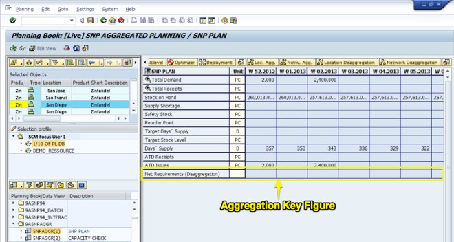
This is the Key Figure in the Planning Book.
Location aggregation is one of three different types of aggregation available within SNP. There is a good deal of confusion even among SNP consultants as to how location aggregation works. The most common requirement for which I have seen location aggregation proposed is for redeployment. Redeployment is a supply planning run that SNP does not cover. (for a full description of redeployment, see the following article)
Aggregation is much less frequently used in supply planning than demand planning. Aggregation in supply planning works much differently than in demand planning software. For instance, while hierarchies and attributes are built right into the Data Workbench in DP and every DP implementation, I am aware of using a hierarchy and most often uses attributes. SNP projects that use aggregation are pretty rare, at least at the sample of clients that I have worked with.
Aggregated Supply Planning and SNP’s Three Methods
Disaggregation takes place with a fair share rule.
Using aggregations in SNP consists of configuring the following areas in a way that works together:
- The Aggregation Planning Area (9ASNP02)
- The Aggregation Planning Book (9ASNPAGGR)
- The Setup of the Actual Hierarchies
- Related Settings Such As the Aggregation Settings in the Following Areas:
- The Transportation Lane
- The Optimization Profile
- The CTM Profile
When aggregation is used, the planners must be trained to use the specialized 9ASNAPAGGR planning book.
The aggregations are set up in /SAPAPO/MSDP_ADMIN, the planning area administration transaction. Here are the steps to set up a hierarchy:
Under the key figure tab, we need to maintain the forecast and stock key figure’s aggregation definition.
- Set the aggregation in the key figure tab of the planning area:
- Choose the aggregation type.
- In the aggregate planning tab, assign the hierarchical structure to the hierarchies that have been created.
- Define custom planning book with /SAPAPO/SDP8B and copy the standard planning book 9ASNPAGGR with two data views SNPAGGR(1) and SNPAGGR(2)
- Assign the new planning area as the custom planning book copies the original planning area 9ASNP02.
- In the planning book maintenance transaction /SAPAPO/SDP8B