How to Understand SNP Optimizer Over Ordering

Executive Summary

• Is The Reason for Over Ordering due to R/3 or SNP?
• Examples of Combined Supposed SNP and R/3 Over Ordering
• Examples of Combined SNP Only Over Ordering
• Overages Caused by Both SNP Purchase Requisitions and SNP Planned Orders
• What Recommendations are in the Optimizer Input Log?
• When in the Time Horizon does Over Ordering Occur?
• Synopsis of the Analysis up to This Point in the Paper
• Similarities Between the Products with High Overages
• SNP Optimizer Over Ordering
• Time Decomposition Enabled

Introduction to Overordering

One thinks of supply planning inaccuracy regarding both equally distributing over and under orders. However, on several occasions, I have witnessed SNP both under and over-order. This is most common when either the CTM or the SNP optimizer is used.

It’s rare for much in the way of comprehensive diagnostics to be run on the SNP optimizer. The way that companies find out about is when planners complain about the results.

I have analyzed the overall system results and found over ordering as high as 50% with the SNP optimizer. Considering how most companies set their unfulfilled demand costs so high compared to other costs, I am surprised it is not higher. (See the problems that companies have in setting costs appropriately in cost optimizers in the post)

SNP creates purchase requisitions and planned orders. According to interviews with planners at one client, I found that they have SNP has been creating overly large purchase requisitions and planned orders since SNP first started being used at this company. There is evidence of this over-ordering in some product location combinations in the planning book. However, it is most clearly evident in a comprehensive way by running reports on the average quantity of overstock versus days under the stock.

We have access to BW cubes through the SAP Business Intelligence plug-in for Excel, and this is how we obtained this data below.

The screenshot below shows the results of this analysis.

This shows that, on average, through five locations, the average percentage of the overage is much higher than the underage. (We initially tried to place all the locations in the BW report but received a maximum capacity limitation, so we reduced the selection down to five locations, which turned out to be manageable.)

Is The Reason for Over Ordering due to R/3 or SNP?

One idea proposed is that this over ordering is due to the purchase requisitions that R/3 creates. However, samples from SNP do not support this idea. Here are a few reasons why:

• There are cases where SNP creates excessive purchase requisitions on days where no R/3 purchase requisitions are generated.
• There are cases where SNP creates excessive purchase requisitions, also to already generated R/3 created purchase requisitions. This is clear from the timing of the purchase requisitions creation (which will be demonstrated below).
  Understanding the Interaction Between SNP and R/3 with Purchase Requisitions

SNP does not convert and then rename R/3 generated Purchase Requisitions to SNP Purchase Requisitions. The same is true of SNP Planned (production) Orders. SNP is set up this way because there is traceability as to what system generated what recommendation. Pre-existing R/3 Purchase Requisitions do affect SNP in that they reduce the size of or, in some cases (that is, when operating correctly), eliminate SNP generated purchase requisitions. That is the summation of the relationship between SNP generated purchase requisitions, and R/3 (MRP) generated purchase requisitions. Therefore when an SNP Purchase Requisitions is viewed in the planning book, the viewer can be certain that SNP generated the purchase requisitions.

Therefore, high SNP ordering is not because purchase requisitions were created in R/3 and were then adjusted in SNP. Purchase requisitions created in R/3 have a specific order category, and any former R/3 or SNP generated purchase requisitions are used to make future SNP Purchase Order recommendations. R/3 cannot force SNP to make bad decisions unless it sends inaccurate data such as the stock on hand.

With planned over ordering and therefore planned overstocking, this issue appears at a casual glance to be not entirely restricted to the SNP optimizer. There are examples of what appear to be R/3 and SNP over ordering together. Examples of this are listed below:

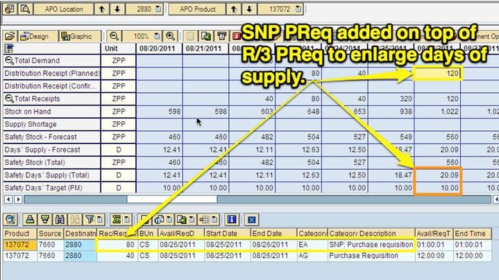
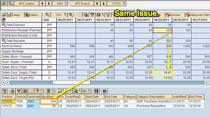
However, the SNP Purchase Requisitions come after the R/3 Purchase Requisitions have already been created upon closer inspection. Therefore, SNP is the system responsible for the over-ordering even though both R/3 and SNP Purchase Requisitions are combined in these screenshots.

Examples of Combined SNP Only Over Ordering

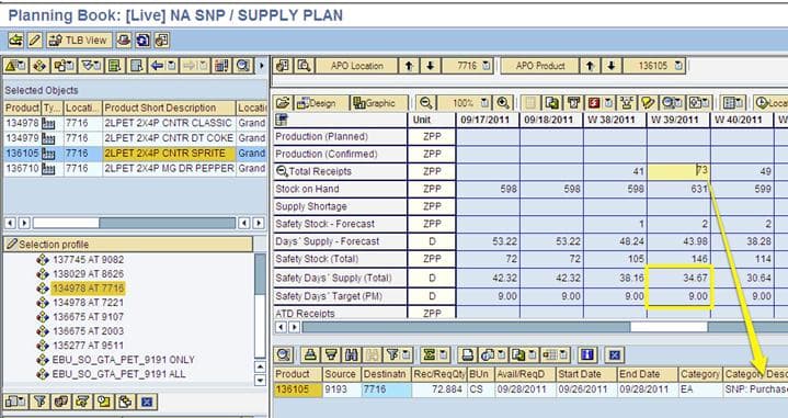
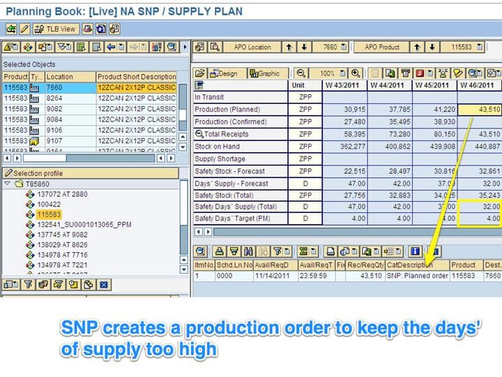
Most cases that have been found show SNP Purchase Requisitions alone and drive up the Days’ Supply far above the target on that particular day. Furthermore, while unnecessary purchase requisitions are the most discussed topic with planners, over ordering with planned orders is also quite common.

Overages Caused by Both SNP Purchase Requisitions and SNP Planned Orders

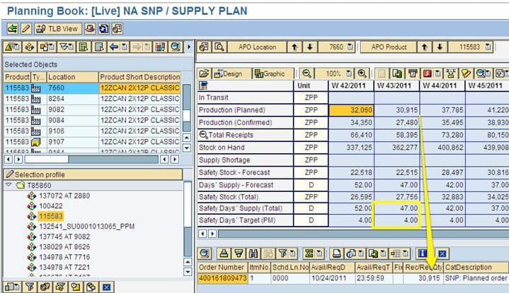
While the primary focus has been on SNP Purchase Requisitions, the overages are related to purchase requisitions and SNP Planned (production) Orders. It is unclear as to why planners do not as frequently discuss this. However, there are some examples of this, and two of them are shown below.

What Recommendations are in the Optimizer Input Log?

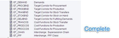
The Optimizer Input Log shows the state before the beginning of the optimizer run. One idea has been put forward that the Input Log should be checked to see if MRP in R/3 created the purchase requisitions that interfered with SNP. At the same time, SAP documentation proposes that the Optimizer Input Log is filled with master data and transaction data. In fact, the Optimizer Input Log is primarily a tool for checking master data. The Results Log, on the other hand, is extensively populated with transaction data. This is necessary to have a comprehensive accounting of the recommendations that SNP created. Checking the Optimizer Input Log categories can validate this.

Once reviewed, it is apparent that this is not where pre-optimizer run transactions are stored. This is shown in the screenshot below:

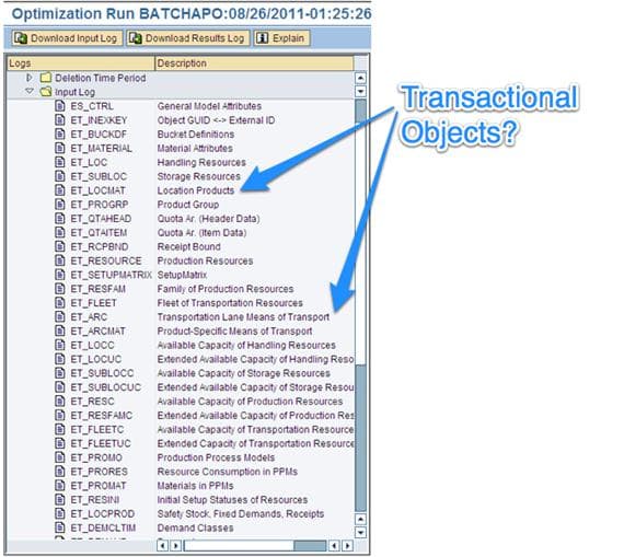
Also, due to the fact above that the order categories already declare their creation system, all SNP versus R/3 generated purchase orders and planned (production) orders can be clearly seen within any view or report generated from APO.

When in the Time Horizon does Over Ordering Occur?

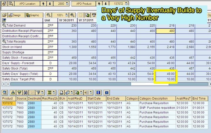
On problem product location combinations, the Days’ Supply continues to build as the timeline progresses. This would imply that the SNP optimizer creates excessive orders only at the end of the time horizon. However, that is not the case. It is only that the later parts of the time horizon show more excessive days’ of supply because it has incrementally built up through excessive orders all along the horizon. However, it is an important point to understand because overages created by either SNP Purchase Requisitions or by Planned (production) Orders that occur later in the planner horizon are not actioned. As time passes later, periods are pulled forward, and the plan is regenerated. Therefore, new and more accurate SNP Purchase Requisitions and SNP Planned Orders are created, and the old, less specific ones are deleted. Because the very high over stocks tend to occur later in the planning time horizon, SNP’s over ordering is less of a concern than if it were more common at the beginning of the horizon.

Another important clue to what is causing over ordering is when the over-ordering occurs in the planning horizon. This is particularly important for cost optimization because cost optimization is often run with a series of different decompositions or divisions of the overall supply network problem. Cost optimization decomposes the supply network problem differently from other methods. The options available within cost optimization are frequently not understood by the client and even the consultant. (to read more about decomposition, see this post) It is important to understand the cost optimization decomposition that is setup in SNP and, in particular, the time decomposition.

Decomposition concerning time means that the CPLEX Optimizer does not process the problem (it is necessary to refer to CPLEX because CPLEX’s makes the optimizer SAP uses — SAP makes no optimizer. This is important because the CPLEX documentation is better than SAP’s, and it is useful to know that you can also use CPLEX help rather than SAP’s help when the question gets into optimization complexity.) Some of the things I learned from this article I read in the CPLEX documentation.

Synopsis of the Analysis up to This Point in the Paper

The following is observed in the system with regards to over ordering:

• SNP consistently over orders
• Over orders can either take the form of SNP Purchase Requisitions or Planned (production) Orders (the fact that both are affected offers clues into the over ordering reason)
• The over ordering is systematic (as demonstrated by the BW report on 5 locations, which compared days of supply to the supply target days).
• R/3 does not cause the over ordering.
  Answering the Question Why SNP is Over Ordering

The next line of inquiry is why over ordering is being caused by SNP. The over ordering observed is not driven by lot sizes as the over ordered quantities are not due to lot size “uplift.” It is not (should not) be driven by costs as the optimizer has a powerful incentive to meet all demands but has no incentive to create excessive orders. For every SNP Purchase Order or Planned (production) Order generated by the SNP Optimizer, it incurs a cost. But if the orders generated are excessive, they do not reduce the costs incurred from unfulfilled demands. Storage costs and production costs are set very low compared to the costs of unmet demands, but they are still costs, and the optimizer is incurring costs when unnecessary, which is not its design. This is resulting in a higher total cost and a less optimal solution.

If costs were driving these excessive orders, a natural question would be why only certain product locations have excessive ordering when unfulfilled demand costs are identical for these product location combinations. The behavior cannot be explained by the SNP Optimizer’s design or by its configuration.

Similarities Between the Products with High Overages

It was observed that all of the examples that have been shown in this document have something important in common. None of them solved optimally. The optimizer solves the supply network problem on the product at a time for each product sub-network. The sub-network is all of the locations, which apply to that particular product. Therefore the SNP optimizer shows very clearly which products were solved optimally and which were not. Furthermore, other sample product location combinations that were also tested also did not solve optimally. These products were randomly sampled.

Of all the products reviewed, all of which contained overages, only the following product sub-problem solved optimally. Roughly 62% if subproblems solved optimally on this particular network optimization run where these samples were taken, and of the 14 products checked (3 in the screenshots + 11 listed just above), the number of products with excessive Days’ Supply (and thus high excessive ordering) is highly skewed to the feasible / non-optimally solved subproblems. Although the relationship is not perfect, it is unlikely that the completeness of these sub-problems’ solution is unrelated to over ordering. In fact, it is the most likely reason for the over ordering.

SNP Optimizer Over Ordering

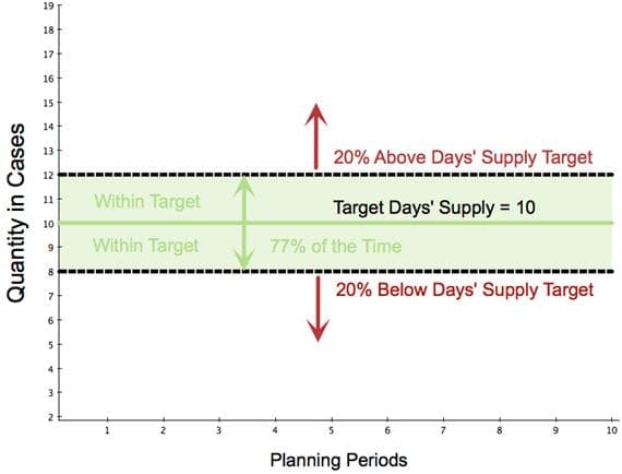
Disproportionate cost setting can be one reason for consistent over or under ordering. However, there are other reasons. This can be learned by analyzing the supply planning output. For instance, the graph below demonstrates overages that are not driven by high unfulfilled demand penalty costs. This is because the overages are not high across the board, but only in a minority of cases.

Time Decomposition Enabled

With time decomposition enabled, the optimizer processes earlier segments of the time horizon first. Sub-problems are given a maximum runtime (a subproblem normally a single product-location sub-network sub-problem – see the article link above for more details). After they reach the maximum sub-problem runtime, the problem is no longer processed. The end state is whatever the optimizer was able to get through. In some circumstances, the sub-problem solves optimally, but sometimes it does not.

On those sub-problems that did not solve optimally, the later periods in the time horizon will be a lower quality solution than the earlier periods as the later periods were less processed or not processed at all. This can be demonstrated by taking a sample of the over ordered products and checking to see if most of them did not solve optimally. If a high number of the product sub-problem did not solve optimally, there is a good chance that this is the problem. Discussions can then commence on making adjustments such as enlarging the processing time window by adjusting the operational workflow, or the easiest and often least expensive alternative, adding more hardware.

Conclusion

While not 100% conclusive, it appears most likely that the over-ordering is due to the products involved being part of sub-problems that did not have sufficient time or were otherwise unable to find an optimal solution. This leads to a recommendation to increase the optimizer’s hardware to solve each sub-problem more fully, if not optimally. Adding more hardware

There are some reasons for over ordering in any optimizer, including SNP. This article has described several things to look for, leading one to determine the route cause. Once the route cause is determined, the solutions become obvious. While the current practice seems to be letting the planners find the solution’s problems, this is not a splendid practice. Diagnostics of the type I described in this article should be run right off the bat when the optimizer is first being tested. Planner input is valuable. However, to get to the bottom of the question, the overall system must be diagnosed in aggregate to determine if the solution is good.