How to Understand The Planning Horizon in SAP SNP - Brightwork Research & Analysis

Table of Contents: Select a Link to be Taken to That Section

Executive Summary

There is a supply planning horizon per planning run, and these changes depending up whether this is the Initial Supply Plan, S&OP, Rough Cut Capacity Plan, etc.
In APO, there is an SNP Heuristic Time Stream, a CTM Time Stream, a Cost Optimization Time Stream, and a Deployment Planning Thread, a Deployment Heuristic, and a Deployment Optimizer.
We also cover the TLB Pull-in Horizon and the TLB Planning Book.

Introduction to the Planning Horizon

Questions of timing are some of the most perplexing in supply chain planning. Considering the interaction between the planning horizons maintained, various interacting supply chain systems are necessary for a proper planning design. You will learn about the planning horizons in different APO modules in detail and their relationship to one another.

Our References for This Article

If you want to see our references for this article and other related Brightwork articles, see this link.

Notice of Lack of Financial Bias: We have no financial ties to SAP or any other entity mentioned in this article.

This is published by a research entity, not some lowbrow entity that is part of the SAP ecosystem.
Second, no one paid for this article to be written, and it is not pretending to inform you while being rigged to sell you software or consulting services. Unlike nearly every other article you will find from Google on this topic, it has had no input from any company's marketing or sales department. As you are reading this article, consider how rare this is. The vast majority of information on the Internet on SAP is provided by SAP, which is filled with false claims and sleazy consulting companies and SAP consultants who will tell any lie for personal benefit. Furthermore, SAP pays off all IT analysts -- who have the same concern for accuracy as SAP. Not one of these entities will disclose their pro-SAP financial bias to their readers.

What is the Planning Horizon?

The planning horizon concept is one of the subsets of planning timing that are necessary for setting correctly. The planning horizon can be challenging to obtain because it must be understood in conjunction with various other settings. Planning horizons also, depending upon the planning horizon, can be set in multiple places. For instance, a CTM Profile is set to run for the background and is set for a specific start date.

Complications of the Interactions Between Multiple Planning Horizon (s)

Difficulties with the interactions between multiple horizons are why Horizons’ issue should be addressed from a comprehensive perspective. One method is to place all the horizons that apply to the project into one document. I find a spreadsheet useful for this task and have included a copy of the planning horizon spreadsheet used on an actual project.

This is an excellent method for providing a shared agreement on the planning horizons and to develop an initial straw man for what the horizons should be.

The Planning Horizon Definition and Logic

Each planning horizon does something different in the system and has different logic for being set. Below the horizons, I have included a section on planning horizon logic, which is an example of why one would set the horizons for a specified duration. To start the process, I will just enter simple logical statements, even though they don’t apply to a particular client. However, after an initial viewing, they can be made more precise. This also dovetails with the inclusion of each planning horizon’s definition so all the participants in planning horizon-setting meetings can fully understand the horizons.

To start the process, I will just enter simple logical statements, even though they don’t apply to a particular client. However, after an initial viewing, they can be made more precise. This also dovetails with the inclusion of each planning horizon’s definition so all the participants in planning horizon-setting meetings can fully understand the horizons.

Supply Planning Horizon Per Planning Run

Four types of planning runs are generally performed in any supply planning system.

S&OP and Rough Cut Capacity Plan: This is used for long-range planning and, in most cases, is an off-line analysis and is not part of the live environment.
The Initial Supply Plan (performed by MRP in ERP systems): Produces the initial production and procurement plan. It is focused on bringing stock into the supply network and on creating inventory with planned production orders. It can also be called the master production schedule (MPS) if the initial supply plan is run under specific criteria.
The Deployment Plan (performed by DRP in ERP systems): Focused on pushing stock from locations at the beginning of the supply network to its end.
The Redeployment Plan (performed by specialized applications with redeployment functionality or with a custom report): Focused on repositioning stock, which is already in the supply network, to locations where it has a higher probability of consumption.

Each planning run has a different planning horizon. I have listed the typical planning horizons below:

S&OP and Rough Cut Capacity Plan: A year or greater
The Initial Supply Plan: Most often a year
The Deployment Plan: Typically, a few weeks
The Redeployment Plan: Typically three to six months

The S&OP planning run, Rough Cut Capacity Plan, and initial supply planning run all use the same three methods available in SNP that create planned production orders and generate procurement recommendations to bring inventory into the supply network. These three methods are:

CTM
The SNP Heuristic
The SNP Optimizer

Deployment is accomplished with either the SNP Deployment Heuristic or the SNP Deployment Optimizer. My editor found this confusing, so let’s list the different methods available for SNP supply planning. There are two for the initial supply plan and one for deployment.

Initial Supply Plan/S&OP/Rough Cut Capacity Plan

CTM
The SNP Heuristic
The SNP Optimizer

Deployment

The SNP Deployment Heuristic
The SNP Deployment Optimizer

Saving as Variants

While the same methods may be used for each planning run, differences in the saved profiles or variants, including but not limited to the planning horizon. As well as different planning runs being performed in different versions—active, inactive, etc. This provides the necessary planning output to meet the needs of each of the planning runs. Redeployment is not a functionality covered by SNP, so I will not include it in this book. For those who are curious about whether one of the supply planning methods can be adopted to plan redeployment, after extensive testing and checking on this topic, I can confidently say that they cannot. For those wishing to integrate redeployment stock transport requisitions from outside of APO and incorporate them into APO, I cover this topic in detail in the book Multi-Method Supply Planning in SAP APO.

Supply Planning Horizon for S&OP, the Rough Cut Capacity Plan, and the Initial Supply Plan

I will start by showing how the planning horizon is set for the SNP Heuristic, CTM, and the SNP Optimizer, and then I will move to the SNP Deployment Heuristic and SNP topic Deployment Optimizer. I will refer to the “time stream in several areas,” which is the official SAP terminology. A time stream applied to a supply planning method is usually that method’s planning horizon.

SNP Heuristic Time Stream

On the screenshot on the following page, you can see how the planning horizon is set with the SNP Heuristic.

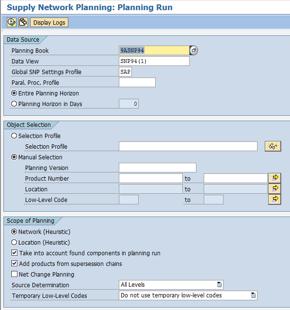
On the SNP heuristic setup screen, an SNP Heuristic Profile can be set to process for up to the entire planning horizon (as set in the Planning Bucket Profile). In that case, one would make the setting the whole planning horizon option. If one wants to run the SNP heuristic for a time horizon shorter than the Planning Bucket Profile (see the Planning Bucket Profile—or time stream for more details), then the second selection would state the planning horizon days.

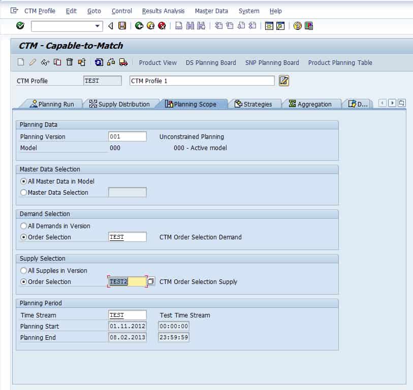
CTM Time Stream

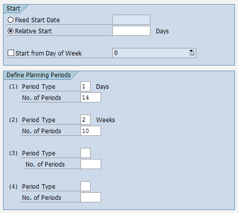
The planning periods are additive and determine the planning horizon of CTM. In the screenshot below, I have created a CTM Time Steam made up of the following combination of periods. This time stream will begin with 14 days and then move to 10 periods of two weeks for twenty weeks.

The timestream can be conclusively shown in a spreadsheet, allowing us to show multiple time stream settings close to each other. This is important because a procedure will often have various runs and numerous time streams. In the example on the following page, we have one CTM Time Stream for a daily CTM run. The weekly run is for the long-range run used in a company’s S&OP process and master production schedule. This is shown in the screenshot below:

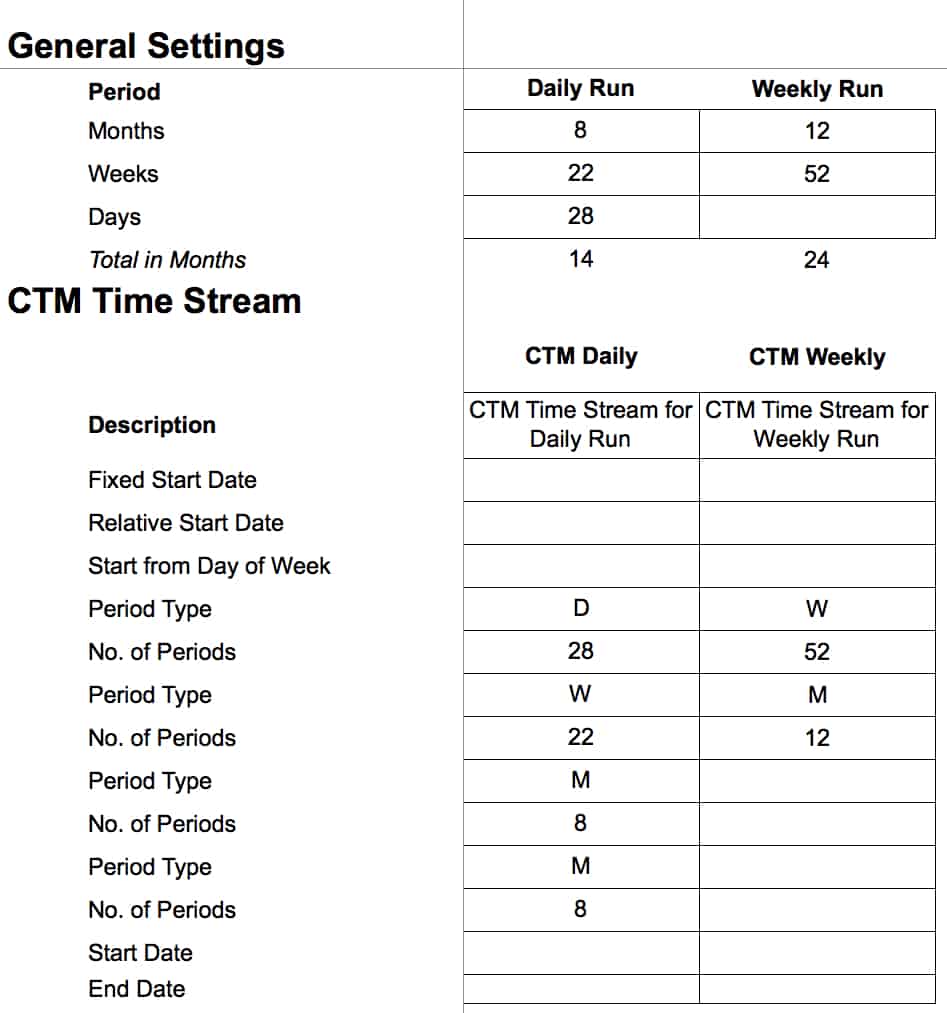
The mini spreadsheet at the top is the simplest way to state the periods and the number of periods. For the daily CTM run, the entire time horizon that CTM will process is fourteen months, and the weekly CTM run is twenty-four months or two years.

Cost Optimization Time Stream

The cost optimizer in SNP is used for both what is referred to as the SNP Optimizer, which is also known as the SNP “network” Optimizer and is used for the initial supply planning run. The same cost optimizer is also used for the SNP Deployment Optimizer. So when I refer to “the SNP Optimizer,” I am referring to the network optimizer, which creates purchase requisitions and planned (production) orders. This is as opposed to the SNP Deployment Optimizer. This is not the most precise terminology I know, but it is the official nomenclature that SAP chose to use. Both the SNP Optimizer and the SNP Deployment Optimizer are set up as profiles.

This allows different variants or different settings for both optimizers to be saved and re-run in the future and for the scheduled variants. The optimizer profiles are broken into tabs, and I have only included the tabs, which have timing settings.

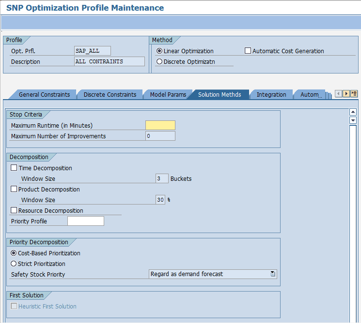
Two-time settings at the top of this tab are related to how many times the optimizer should process or how long the optimizer should run. Optimizers must be capped because they will continue to run unless told when to stop (optimizers will also eventually stop when they reach the objective function—or the “optimal” solution—is reached).

However, in most cases, the optimizer must be stopped well before it meets its objective function. The complexity and processing time for supply chain optimization make it impossible to finish in a time that fits within the available processing window.

The Solutions Methods tab in the SNP optimizer allows the use of time decomposition, which is the most common type of decomposition. Time decomposition divides the problem into segments, which the optimizer then processes separately. For instance, if the time decomposition is set to “3,” then the defined planning horizon is segmented into three components (from recent to further). The nearest planning time segment is processed first. Optimization decomposition is one of the most important things to understand about optimization and is described in more detail in the article.

Three timing settings on this tab tell the optimizer if they should use the SNP Production Horizon, the SNP Stock Transfer Horizon, and the Forecast Horizon that are the Product Location masters. I discuss each of these horizons so that I won’t cover them here. The most important thing to understand is that specific optimizer runs can be made to ignore these values.

The Deployment Planning Thread

In SNP, confirmed the deployment planning run only creates sTRs. The deployment planning run follows the initial planning run and moves stock through the supply network. Deployment uses the initial supply plan to determine the strategy for moving projected inventory on hand through the supply network. The Deployment Plan (performed by DRP in ERP systems) is explained in the article.

Now we will get into the various horizons of the deployment planning run.

The Deployment Heuristic

As with the initial supply planning methods, planning horizons are assigned to the deployment heuristic and the deployment optimizer profiles/variants.

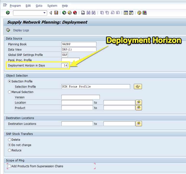
The deployment heuristic uses a deployment horizon, which is stated in days and is shown above.

The deployment heuristic has very few settings overall and just one time-related setting.

The Deployment Optimizer

The SNP Deployment Optimizer is very similar to the SNP Optimizer with two critical differences:

It does not include any production settings; that is, it does not read PPM/PDSs and does not offer discrete optimization options for production parameters.
It has a special tab for deployment parameters that the SNP Optimizer does not have.

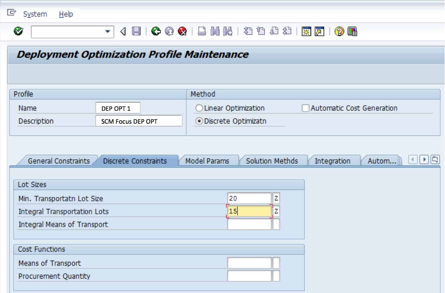
Notice there are no production settings on the discrete optimization tab.

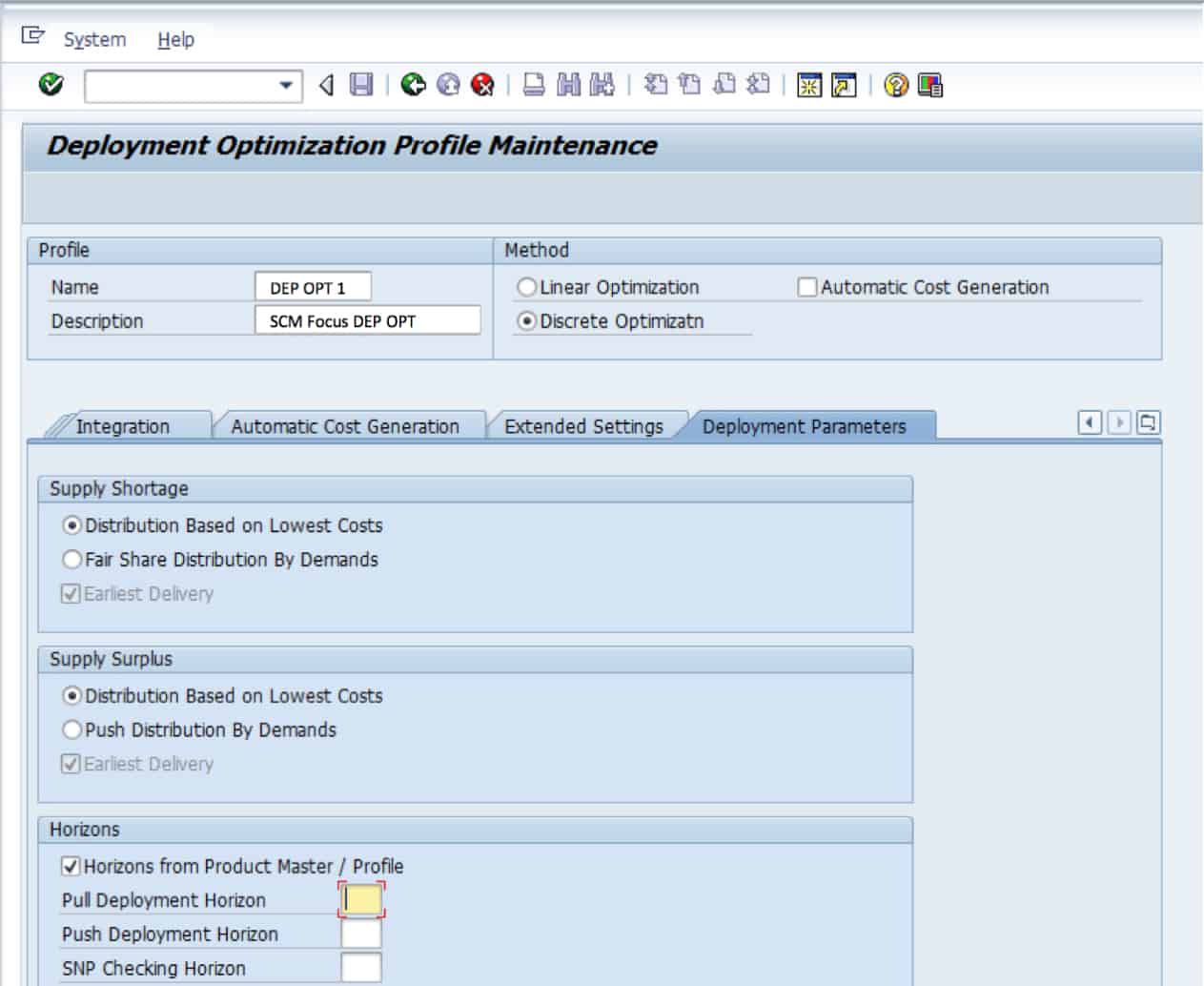
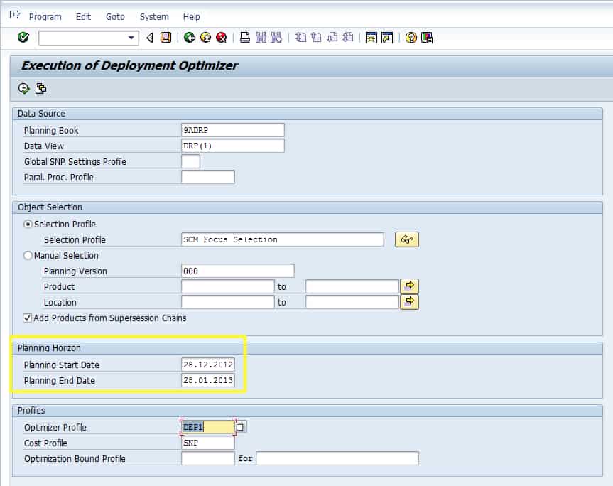
As with the SNP Optimizer, the SNP Deployment Optimizer can be run in the background and can have its planning horizon defined in a variant. This variant can be scheduled and run automatically and repetitively.

Other Deployment Time Settings

These deployment settings are on the SNP 2 tab of the Product Location Master, which I will cover in detail in the following section. These deployment timing fields are described below:

Indicator—Real-Time Deployment

When activated, the deployment is based upon the most up-to-date planning results from the initial supply plan. This is used for fair share distributions. However, the real-time deployment does not consider quota arrangements or even the transportation lanes and any location other than the source specified. Therefore, stock transfers are only created between the deployment source location and the destination location.

Distribution

Where you state if you want to push, pull, or push/pull distribution. With push distribution, deployment pushes out all stock within the planning horizon. With pull distribution, nothing is distributed to the demand location before the need date. With push/pull distribution, the material is moved immediately as with push—but for the pull horizon.

SNP—Checking Horizon in Days

This is an optional setting. It is used in deployment, both in the SNP Deployment Optimizer and in the Deployment Heuristic. This setting controls how the available-to-deploy quantity (ATD) is calculated. When enabled, the ATD for the push deployment horizon is reduced. It is a signal for the system to add the ATD receipts for the current period and the prior period and remove all ATD issues within the checking horizon. When not specified, the system adds ATD receipts of the current and past periods and eliminates ATD issues.

SNP Stock Transfer Horizon (on the SNP 2 tab of the Product Location Master)

The SNP Stock Transfer Horizon controls both when the unconfirmed STRs are generated (they are created during the initial supply plan and transfer distribution demand through the supply network). And when the confirmed stock transfer requisitions are created (they are generated by deployment). The question of an unconfirmed versus a confirmed STR can be a point of confusion. Why would anyone need an “unconfirmed” STR? This is because SNP needs a method of creating distribution demand and distribution receipts in a supply network. SAP could have named this object several things but settled on “unconfirmed” STR. A confirmed STR results from a deployment run (either the deployment optimizer or the deployment heuristic).

The SNP Stock Transfer Horizon control is helpful in essentially disabling SNP over a particular duration. I have used it in the past when Kanban is configured in SAP ERP to handle stock movements that are in the short term (say fourteen days out), with SNP taking over the planning after fourteen days. However, generally speaking, this setting is not used that frequently.

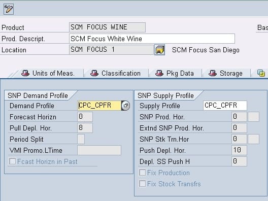
The SNP stock transfer horizon and its relationship to the SNP Planning Horizon are described in the graphic below:

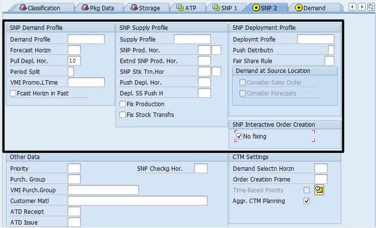
Understanding the Time Settings and Profiles on the SNP 2 Tab

All of the supply planning methods use the fields on the Product Location Master, and most fields are on the SNP 2 tab. While this is a well-known tab, the more one analyzes the time settings on this tab, the less logical the organization of the fields within the tab’s various areas appears. There are three profiles on the SNP 2 tab, as follows:

SNP Demand Profile
SNP Supply Profile
SNP Deployment Profile

The profile is an essential way of controlling master data. A master data profile is simply a collection of master data fields related and can be saved as a group or variant.

Most Master Data Fields

Of all the APO modules, SNP has the most master data fields, explaining why SAP development was so liberal in applying the profile concept to SNP master data fields. For instance, when a profile is saved in the SNP Demand Profile, the user has the option of filling in five other fields. Whenever this SNP Demand Profile is applied to a product-location combination, all of the applicable fields in the product location are populated at once. The fields for each of the profiles on the SNP 2 tab are shown on the following page:

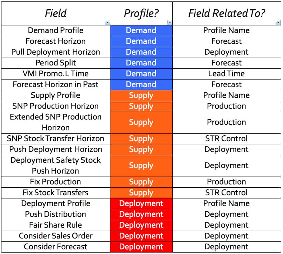
Even though each field is assigned to a specific profile on this screen, the profiles are simply a way of grouping the fields. The fields can be grouped under other categories (such as function or purpose). If the same list above is sorted by what the field does or what it is related to, the list looks like the following:

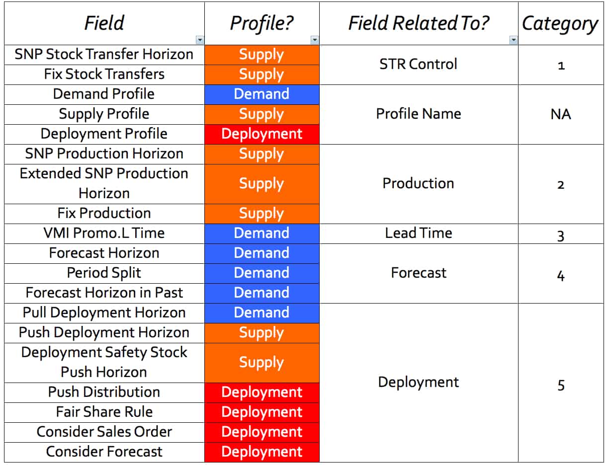
I have placed the fields into five categories: STR control, production, lead time, forecast, and deployment. I don’t include the profile’s name as a category, as it merely serves to group the associated fields. If one looks at the profile column, it should be apparent that different categories of fields (from a functionality perspective) are somewhat mixed up among the three different master data profiles. However, one shouldn’t assume that all fields that control the timings for a particular functionality area, even within the SNP 2 tab, are in its named profile. Furthermore, there are fields (such as the SNP Checking Horizon) that should be—or at least could be—part of the SNP Deployment Profile but are not.

The Functionality of the Timing Fields

Rather than discussing the timing fields by their appearance in the user interface, I wanted to discuss them by functionality. Doing so meant drawing upon different fields from different profiles. Consider this when viewing screenshots included in this book as we discuss the different timing categories. Throughout the book, rather than repeatedly showing the SNP 2 tab, I will ask you to refer back to the following screenshot to get your bearings about where the fields I am discussing are located.

Forecast-related Supply Planning Timings

SNP requires its timing settings for how to work with the forecast. The following fields on the Product Location Master control the timing settings.

There are three fields on the SNP 2 tab that control the use of the forecast by SNP.

Forecast Horizon: Horizon in calendar days during which the forecast is not considered part of the total demand. Supply Network Planning (SNP) does not consider the forecast within this horizon when calculating aggregate demand. Outside of this horizon, the system calculates total demand using either the forecast or sales orders (whichever value is more significant) and the other demands (dependent demand, distribution demand, planned demand, and confirmed demand).
Period Split (the official field name being Time Based Demand Distribution [Period Split]): Defines how planning data is disaggregated when you release the demand plan from Demand Planning to Supply Network Planning. The options are blank—The data is disaggregated and released to all of the specified horizon workdays. “1”—The data is disaggregated to all of the workdays in the specified horizon but released only for those days that lie in the present and future; “2”—The data is disaggregated to the workdays in the present and future, and then released for the same days.
Forecast Horizon in Past: If you do not specify a value for the forecast horizon or enter the value 0 and set this indicator, the forecast horizon’s consumption logic also applies for planning periods situated in the past (before today’s date). This is a somewhat convoluted way (Yes, the first part of this definition is from SAP—can’t you tell?) of saying that just as with the Forecast Horizon (in the future), the Forecast Horizon in the Past controls if the forecast is included in the backward consumption. This is a strange setting because if one does not want to perform backward forecast consumption, don’t use forecast consumption. I am not sure why I would ever want to enable this field, and I can’t recall seeing it used for any of my SNP clients.

What the SNP Forecast Horizon Determines

The SNP Forecast Horizon determines what is included as demand. This setting’s primary use is to remove forecasts from the nearest period, the logic being that if the sales order has not materialized within. For example, the time period of one or two weeks out from the current day, it is unlikely that it will materialize at all (of course, this very much depends upon the situation, as many companies receive sales orders up to the current day).

This setting prevents the company from building inventory that may not be consumed. Because this setting is at a product location, the company can use it selectively for the product locations for which sales orders come in “x” number of days before the current day (where “x” is the duration of your choosing).

Planning Calendars/Time Streams

This is a good point in the book to move to plan calendars/time streams. The planning calendar/time stream defines the following time information:

When the time stream begins (either a specific date or a relative start date).
The length of the duration, in periods.
The different duration period types (days, weeks, months).
How many different duration period types will be in the time stream?
The sequence of the different duration period types.

Calendars/time streams in APO can be created in either the APO configuration or the SAP Easy Access menu with the transaction /SAPAPO/CALENDAR. The planning calendar/time stream user interface is a bit unusual in that it can create a CTM time stream or a standard planning calendar/time stream. If a CTM time stream is selected, the options look quite different from if the standard planning calendar/time stream is selected.

In this screenshot, we create a time stream/calendar for production. The options listed above are used to set up the CTM time stream. How the time stream sequence is built is described in the article.

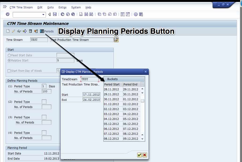
This screen serves as a quality check to ensure that the right periods are created. Within Time Stream Maintenance, one can select the Display Planning Periods button, which is useful because the time stream maintenance transaction is not particularly user-friendly.

When creating a standard planning calendar rather than a CTM time steam, the following options are available:

On this screen, I can name the calendar, define how far into the future I would like the calendar to be valid, give it a time zone, state whether it is a working time calendar or a period calendar, and then assign a factory calendar to it.

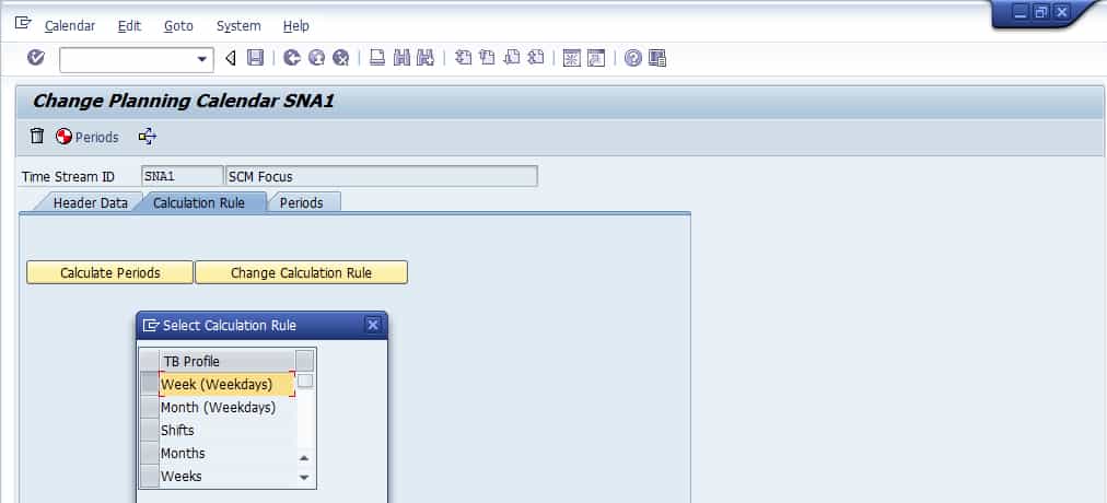
On the second tab, I have to define a calculation rule, which chooses the calendar’s periodicity.

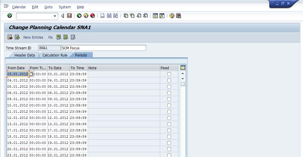
The third tab shows all of the specific valid time periods that have been created from the previous tabs.

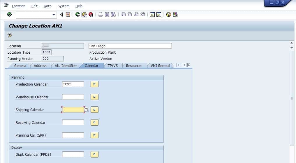
Now we assign the time stream to the location, which controls the timing for the location. Six different calendars can be associated with a location. These calendars control various aspects of the location’s behavior.

What Calendars Enable

The calendars tell SNP and PP/DS which days are available for planning in the factories and the distribution centers. The location calendar is the parent object, and then within the calendar, the resources are the children, and they place a further constraint on capacity.

Supply Planning Timings Related to Lead Time

There are various lead times in any supply planning system, but the most prominent are the lead times for procurement, production, and stock transfer. While there are several important aspects to lead times, only one is focused upon: the actual duration of the lead time. The supply planning methods in SNP do not always consider the lead times entered as master data. How the lead times are treated depends very much upon the scheduling direction of the supply planning method used to plan the product location.

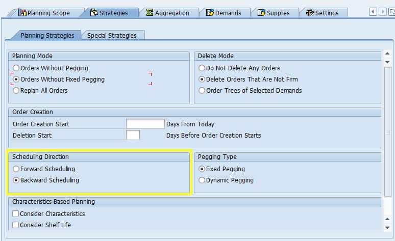
Each supply planning method can be scheduled either forward or backward. This is the scheduling direction setting for CTM. Constrained methods can use the backward or forward option. Unconstrained methods have the third and often default option, which is first backward and then forward.

When the scheduling direction is set to backward in the Product Location Master, the lead times control when scheduled, when the scheduling direction is set to forward, lead times are not factored into scheduling, and every demand is scheduled as soon as possible.

The TLB Pull In Horizon

One area that is confusing in SNP is the interaction between the Transportation Lane and the TLB profile. This confusion is enhanced because several settings seemed to have been destined for the TLB profile that instead was placed on the transportation lane.

The Benefits of a Many to Many Relationship

The association between the TLB Profile and the Transportation Lane is straightforward. It is many to many. However, several fields are assigned to the Transportation Lane that really should have logically been applied to the TLB Profile. One notable field which was mistakenly assigned to the Transportation Lane is the Pull-In Horizon. The Pull-In Horizon declares to the system how far out to look to pull in STOs. This is why it is strange and even ridiculous that it was placed on the Transportation Lane. By putting here means that each lane can only have one Pull In Horizon when placed on the TLB Profile, the horizons could be more flexibly managed. Why SAP? Why did you do that?

TLB Pull In Horizon Versus the Supply and Demand

Two settings that are essential not to confuse with the TLB Pull In Horizon, but which is very easy and natural to confuse with, are the Push and Pull Deployment Horizon, which controls how far out the deployment runs.

OF COURSE, the TLB Pull-in Horizon is not related to this strictly for the STOs that are pulled into the TLB optimizer.

TLB Pull-in Horizons and the TLB Planning Book

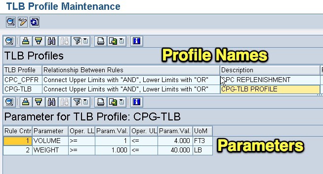
The Pull in Horizon eventually ends up in the TLB Planning Book, which can be seen when one brings up the parameter screen. This can be done by selecting the “face” button in the TLB Planning Book.

This brings up the parameter screen below.

This can be easily manually overwritten. Some people confuse the Pull-in Horizon for the initial data selection period. However, that is not right. The TLB Planning Book horizon controls the data selection period, and this is the initial stock transfers brought into the system to be load built.

The Pull in Horizon is used when a full truck can be build by going beyond the dates in the initial selection period. The best way of thinking of the Pull-in Horizon is to “top off” existing loads that are requested to be built. So if you want to develop the load today, you have enough volume to fill two trucks. The Pull-in Horizon suggests other, usually smaller quantities you can bring in to top off the trucks to not shipping as much space and better utilizing the truck. It is a form of over shipping. This can be a concern for companies that do not want to over ship, as they may need the product at the current location to bring in another demand from another location.

SAP’s Definition of the TLB Profile

The number of days from the current date in which the Transport Load Builder (TLB) can take into account existing deployment stock transfers when constructing TLB shipments, if it cannot use the deployment stock transfers for today’s date to load a means of transport within the valid parameter limits. The TLB takes into account the pull-in horizon when it performs a shipment upsizing. The system uses this method to attempt to avoid remainder quantities that do not fall within the valid parameter limits for a shipment. The system upsizes the quantities to be shipped, by adding demands that fall within the pull-in horizon. Your Customizing settings decide whether the TLB performs a shipment upsizing. You make these settings in the fields for the transportation lane Siz.Decsn (decision basis for shipment sizing) and Siz.Thrhd(threshold value for shipment sizing).

Concerning the last part of this, the location of Siz. Descn and Siz.Thrhd, if anyone knows where this is, write a comment below because I have not been able to find these fields.

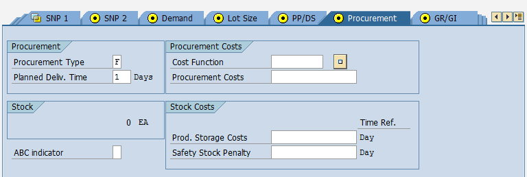
Planning Delivery Time in Days

Planning delivery time is the lead time associated with external procurement, one of four options for the Procurement Type field on the Product Location Master. These options, which are listed below, can be set for any product-location combination.

External procurement
In-house planning
External or in-house production
External procurement planning

The Procurement Type is the primary setting for whether a product is produced internally, procured externally, or both. Production occurs in internal locations, and in most cases, externally procured products will be produced by vendors/ suppliers that are not modeled as SNP locations. When this is the case, the lead time is taken from the Procurement Tab of the Product Location Master. However, a vendor may also be set up as a location in APO. I cover the alternatives in this area in my book, Setting up the Supply Planning Network in SAP APO, so I will not cover that topic.

The lead times are, of course, significant input into planning systems, as they determine when supply chain planning requisitions need to be created.

In most cases, the planning method is set to backward scheduling, which means that the calculation of dates for planned orders (which convert to either a production order or purchase order) and stock transfer requisitions is based upon subtracting the lead times from the need dates. SNP lead times include the following:

Inter and Intra location lead times (which include procurement lead times and internal location-to-location lead times).
Non-production location processing times (goods issue, goods receipt)
Production lead times.

The Problem: A Problematic Deployment Solution

Many years of using SAP APO deployment have me questioning why APO should be used for deployment. The reason is that it is far more straightforward to build a custom deployment solution from scratch that has to deal with SAP’s deployment functionality continually. The deployment solution is better and more effectively run from a cloud service provider and connected to APO, rather than adding the application logic to SAP. We follow the same approach when customizing MRP, as is covered in the article Real-Time MRP.

Deployment in SAP has considerable overhead and does not work the way most companies want to deploy. This is because companies want to fair share stock to downstream locations. The optimizer states that it does this, but after years, most companies have either given up on the optimizer in SAP or are still struggling to get it to work and have spent enormous sums and still have reduced quality output. SAP’s deployment optimizer does not make any sense and will never work correctly, as we covered in the article The Problem with SNP Optimizer Flow Control.

The master data maintenance in the transportation lanes, the failings of the deployment optimizer, and the overall overhead are merely unacceptable for the output produced by SAP APO. APO’s deployment heuristic works but is so basic that it can be easily replicated by far more comfortable to use externally developed solution that allows the solution to be customized for the requirements. Deployment functionality offers no reason to use it, other than it is “SAP.”

Being Part of the Solution: Running Deployment Externally

This article has been written for people that have to get deployment to work in APO — but it is not a very good solution. The best solution is to run the deployment externally and then import the data back into APO — or even APO and import the data into ECC. The application runs on AWS, and so we can bring large amounts of server resources to the problem and run it far more quickly than any SAP server that currently runs APO can.

If you are interested in doing this, contact Brightwork. We have a ready-to-use deployment optimizer with logic for deployment that is easily adjusted and can eliminate APO deployment problems. Some work in making alternations for the requirements, but it can easily beat output produced from APO. And it is a great way to re-establish credibility with the business.