How to Perform Cost, Duration and KPI Production Scheduling Optimization
Executive Summary
- There are many ways to perform optimization for production scheduling.
- We will cover three different ways, cost, duration, and KPI.

Introduction
In this article, we will cover three ways of running optimization for production scheduling.
Cost Optimization
Cost-based optimization or cost minimization has been the most common way to perform production planning and scheduling optimization. However, duration or time optimization offers some very significant advantages over cost optimization.
- It’s easier to agree on times than costs.
- The actual objective of companies usually is to minimize times while meeting demand.
However, while cost optimization tends to be set once and often not changed for years, PlanetTogether’s duration-based optimization engine allows for different weights to be applied to various factors such as setup hours or delivery date. (show optimization rule) These optimization rules fall into the following categories:
- Delivery Date
- Priority
- Efficiency
- Operation Attributes
- Material Groupings
- Ranges
Scenarios can be compared for how they differ with the compare scenarios screen. (Select compare scenarios button). Secondly, what-if scenarios can be switched to live and vice versa.
Capabilities are flexibly assigned to resources in PlanetTogether. The schedule can be optimized and analyzed as to how the additional resources will impact the schedule.
PlanetTogether can take material and finite capacity into account simultaneously without the necessity of two steps. Secondly, what is shown in terms of material and inventory constraints is very flexible. PlanetTogether allows for bottlenecks to be seen in the multi-level bill of materials through the use of the Connected Job Gantt, which can be accessed from the Gantt’s operation right-click menu.
Compatibility Constraints
PlanetTogether can handle requirements where the material is compatible with the materials being run on other resources. This is generally important in process industries. Called Compatibility Constraints in PlanetTogether, they can be set up in the following way:
Select the compatibility group to which the resource belongs in the Resource Properties
The job operation must specify the compatibility code for the resources to be scheduled based upon the specific compatibility.
Compatibility Groups as Assigned to Resources
Each manufacturing order has one or more alternative paths in PlanetTogether. If there are multiple ways of making a product, then an alternative path can be created for each method. Each manufacturing order has one default path, which is always used during the optimized process. From the Gantt View, you can manually drag and drop the job onto a different path by using the alt key and dragging the activity blog.
What is Throughput Accounting?
Throughput accounting is based upon a simplification of accounting designed to provide more accurate levers for management to drive decision-making.
In this context, “throughput” is an extension of the original word, which normally means
“the amount of material or items passing through a system or process.”[1]
However, as applied to accounting, it is a measurement of how the entity attains its goal. A goal is generally financial, such as profits or sales. Throughput accounting was developed in the 1980s for a modern set of assumptions versus cost accounting. As such, the two accounting methods have vastly different orientations. Throughput accounting tracks far fewer costs. In fact, under throughput accounting, the only cost categories are expenses and investment.
Throughput Accounting Versus Cost Accounting
The alternative to throughput accounting is cost accounting, which is the accounting method used by companies and finance and accounting functionality in ERP systems. It is also the method of accounting with which people with exposure to business are most familiar. When one states that they have “studied accounting,” normally, what they mean is that they have studied cost accounting.
Many have argued that cost accounting is a dated accounting technique that ultimately drives the company’s counterproductive decisions. To understand why it’s important to understand cost accounting’s origin – and what follows is a brief overview of cost accounting history.
Considering the History of Cost Accounting
Some of the current cost accounting approaches are generally thought to have developed around the 1300s and others around the Industrial Revolution (generally considered to have taken place from approximately 1760 to 1870).[2]
While rarely discussed, a major part of the developed world’s standard of living is based upon the productivity gains that trace their origins back to the Industrial Revolution. Many journalists, intent upon overestimating the importance of current times versus past times (a constant interest in writers from any era), greatly misinform their readers when promoting the concept that the modern age has more productivity growth or improvements than the period of the industrial revolution. The data is clear that no subsequent technology revolution has profoundly impacted the standard of living of countries, which industrialized as the improvements that came from the first and second Industrial Revolutions. Some journalists and or business leaders don’t seem to understand what the industrial revolution encompassed. On one technology video, which was playing on a loop at the Computer History Museum in Mountain View, California, covering the history of Silicon Valley, a business leader states that the current innovation in Silicon Valley was the most important development in productivity improvement since the Industrial Revolution when a waterwheel was connected to factories to power them. That statement is incorrect. That description is not a feature of either the first or the second industrial revolution. Water wheels go back at least until the 12th century, preceding the first Industrial Revolution by more than six hundred years. The Industrial Revolution was using fossil fuels to power both manufacturing and transportation technologies. It did not have anything to do with water wheels. Many productivity improvements ranged from 1760 to 1870; however, some of the improvements that are restricted to manufacturing are listed below.
- Fossil Fuels: The use of fossil fuels in the production process
- Steel Production: The ability to mass-produce steel (related to point one)
- Interchangeable Parts: The use of interchangeable parts was critical to keeping machines up – and as machines become able to produce more, keeping them running more important than ever.
- The Powered Assembly Line: Assembly lines existed before Ford, but it was unit drives that allowed distributed electrical motors to perfect assembly lines to quickly and easily bring the work right to the operation work center.
And in addition to significantly enhanced productivity, the Industrial Revolution created the need for accounting for manufacturing activities. The Industrial Revolution marked the first use of the terms “variable costs” and “fixed costs,” which are now embedded within our vocabulary. Cost accounting is essentially a combination of accounting methods that were most appropriate between two hundred and fifty and one hundred and forty years ago for attempting to account for activities and costs.
How Dated and Counterproductive is Cost Accounting?
There are several arguments against the continued use of cost accounting for corporate decision-making. One of the most common arguments is that it is dated and based upon more valid assumptions in a different era.
Some examples of these out of date assumptions are the following:
- Information Access: One example of a profound change is this book’s topic: the access to information that computerization has provided to companies. Cost accounting was developed before computerization. There was a much smaller ability to record and analyze costs than there is today.
- Cost Orientation: Cost accounting was developed to report on the company’s activities, and of course, to pay taxes. Cost accounting was never designed principle to improve decision-making.
- Resource Allocation: Cost accounting encourages behavior that can be counterproductive to the overall organization, to improving throughput, and to redirect resources to activities that enhance some sub-segment of the firm’s performance.
- Arbitrary Overhead Allocation: There is little logic for allocating things like overhead and dramatically changing how a department or activity is perceived. Therefore, future resources it may be allocated. A change in how overhead is allocated can very quickly change the profitability of a department. Cost accounting-based overhead allocation affects much more than planning and scheduling but is a primary reason for the misinterpretation of the actual costs associated with manufacturing outsourcing. This is explained by Dr. Hart Smith in an internal paper written for Boeing related to manufacturing outsourcing.
“Out-sourcing is commonly looked upon by management as a tool for reducing costs. But the unresolved question is “which costs?” In addition, there is the matter of “what is the effect on overall costs?” The first issue to be examined is precisely what is out-sourced and what is inevitably retained. The superficial perspective might be that every internal activity that used to be related to a task that has been out-sourced is no longer necessary. Even that is not true but, worse, it fails to acknowledge all of the new internal tasks that had not previously existed. To add insult to injury, contemporary accounting practices do not allow these unavoidable additional costs to be billed for that particular item of work – because it is no longer identified as an in-house task – so these charges are allocated instead as overhead to any remaining in-house work. This misrepresentation of true costs furthers the illusion that outside production is cheaper than anything done inside, building the pressure to ship even more work offsite, until there isn’t any left. The irony of this situation is that it is so easy to understand in the extreme. Suppose that a manufacturer had succeeded in outsourcing all of the work that it wished to isolate from the preferred task of systems integrator. The allocatable costs from the huge amount of out-sourced work will now appear as overhead on the few remaining tasks, like sales and product support, confirming that these were now even less profitable than manufacturing had been when the spiral began!”
Cost Accounting and KPIs
Cost accounting is similar to various key performance indicators KPIs used by companies that don’t translate very well into meeting the company’s goals. One example is the measurement used by some metals companies of “amount of liquid metal poured per employee.” This is an attempt to develop a relevant metric, but such a metric easily could be gamed. This would be an indirect KPI. However, why use indirect KPIs when direct KPIs can be used instead?
These indirect KPIs are all around us, and we often don’t stop asking what is being measured. For instance, how often have we all heard the quotation the status of the “Dow Jones Industrial Average?” If it goes up, we are told that it is good, and if it goes down, we are told it is bad. However, what is the Dow Jones Industrial Average? The “Dow” was created back in 1896 – of course, pre-computers, to have an index or shorthand for the stock prices of the 30 largest companies in the United States. The lack of computing power availability was instrumental in the Dow and Jones Company in selecting such a small number of stocks – it is easy to compute by hand. However, in the modern era, with computers able to create an index for the entire market and calculate it substantially instantaneously, why would anyone continue to use an index developed almost 130 years ago before a single computer existed?
The unfortunate conclusion I have come to after analyzing many supply chain planning applications is that most software vendors have given little thought to aligning their software with the business objectives, choosing indirect drivers for their software. However, this unfortunate situation should not stop companies from seeking out software that provides simple and direct leverage over what drives the software to make decisions because those software vendors do exist. Throughput accounting allows the software to be adjusted in just such a fashion.
Throughput accounting is focused on attaining the maximum utilization of a company’s resources. This dovetails quite nicely with a production planning system, which has the same focus. The best way to understand throughput accounting is an example.
The book SuperPlant: Creating a Nimble Manufacturing Enterprise with Adaptive Planning Software explains that with Galaxy APS, production resources may be either inside or outside of the company – that is, they may be owned or “rented” resources. When throughput accounting KPIs are combined with superplant functionalities, we have implemented this concept, which can be automatically and repetitively performed in a way incorporated directly into the planning process. Because of this, PlanetTogether recommends to their clients that they use throughput accounting KPIs to drive its production planning and scheduling optimizer.
How Financial Considerations Impact Supply Chain Planning
Before we get too far down the path on throughput KPIs and how Galaxy APS manages them, let us review how financial considerations can directly be made to impact supply planning and production planning applications. Financial considerations have controlled supply and production planning, primarily in the following ways:
- Cost Optimization: This is a major method of supply and production planning and has, of course, already been discussed.
- Inventory Optimization: This supply planning method requires that service levels be placed into the application, which will then drive the application to hold a certain level of inventory –which of course, has a financial cost.
- Target Days Supply: This is a way of setting inventory levels, which considers the cost to keep inventory.
Of the three methods listed above, cost optimization is the most direct manner of driving the planning system output through financial considerations. Cost optimization has been the dominant form of supply and production optimization since many vendors broadly introduced optimization in the early to mid-1990s. Surprisingly, the story about how consistently cost optimization has failed to help companies meet their projects’ objectives is largely untold, although it is quite well known among experienced implementers. While Brightwork Research & Analysis is a few entities to write about this subject, it’s certainly no secret among those with cost optimization implementation experience. However, if you search for books and articles on cost optimization, they almost universally describe how optimization can be used to improve planning at a company, with little to no coverage on the reality of cost optimization projects.
There is quite obviously little interest in explaining the fact of optimization – which at this late date, more than twenty years after cost optimization was first implemented broadly in packaged software, cannot be chalked up to the technology is new.[3] We will spend a little time on this topic before discussing how costs and financial data are covered differently with more nuanced software design.
Cost Optimization as Generally Implemented
The objective of cost optimizers is to minimize costs (although some can maximize profits, this is a bit hypothetical as costs are rarely used in this manner).
The original idea was that somewhat actual costs would be utilized. The optimizer would trade off the various costs to develop the most cost-beneficial solution for the company.
As it turns out in practice, not only are the costs entered into cost optimizers not “accurate,” they are often not even proportional to one another. How disproportionate are they? Well, here are some examples of costs for one client.
- *Storage Costs: 1 to 10 depending upon the location
- Delay Penalty: 3,300 to 5,500, depending upon the product-location combination.
- Penalty for Non-delivery: 3,300,000 to 5,500,000
- *Transportation Costs: Zero
- Safety Stock Penalty at All Locations: 1,400
- *Production Costs: Zero
*Those costs with asterisks decrease the incentives to build stock. Those without asterisks increase the incentives to build stock. All of this client’s cost settings are set to increase stock.
Obviously, the non-delivery penalty costs are set 1000 times greater than the next closest costs, which are the delay penalty costs. And this leads to an important discussion as to the categories are costs that are used in a cost optimizer.
Costs can be neatly divided into implicit and explicit costs. Explicit costs are those costs that the company incurs. This includes costs like Transportation Costs, Production Costs, and Storage Costs. Implicit costs are costs for which the company can find no invoice but which “count.” Good examples of costs within this category are the penalty costs.
- Three of the implicit costs listed above (the Delay Penalty, the Penalty for Nondelivery, and the Safety Stock Penalty) are all set very high then the other system costs. This will provide a strong incentive to carry a lot of stock.
- All of the explicit costs listed above (Storage Costs, Transportation Costs, PDS Costs) are either set to zero or set so low that they can’t influence the solution. Optimization is supposed to allow for the intelligent trade-off of different costs to meet the implementing company’s specific business requirements. However, with the system’s costs, the optimizer will only drive to service level and inventory in-stock positions without considering the costs to serve.
In addition to the “costs” being developed with very little logic, I have observed no or meager costs in the explicit costs. The costs set extremely high for the implicit costs — those which are associated with the service level and maintaining stock. Here is another example from a different client.
- Storage Costs: 100 to 140 (depending upon the location-product combination)
- Penalty for Non-delivery: 75,000 to 95,000 (depending upon the location-product combination)
- Transportation Costs: 1 to 3 (depending upon the model)
- Safety Stock Violation Costs: 200 to 350 (also depending upon the location-product combination)
- PDS (Production) Costs: 1 to 4 (depending upon the product line combination)
Here the implicit costs are much lower than in the first example. The transportation costs and production costs exist, although they are still quite small. The storage costs are finally approaching the level where they put a true restriction on holding stock.
Analyzing Costs Used in Optimizers
At company after company, the management questions what the optimizer is doing. However, it is not only the management; often the business, that has to work with the poor quality output has similar questions. Many times implementing companies demonstrate little interest in evaluating the costs that are driving the optimizer. Often people involved in the implementation at companies refer to cost optimizers as “black boxes.”
When I extract the costs incurred, I find that the costs driving the system at various clients are just a few of the possible costs. For instance, in SNP, the possible costs that can be incurred are the following:
- SNP Profit
- Total Costs in Objective Function
- Total Production Costs
- Total Procurement Costs
- *Total Storage Costs
- Costs for Extending a Resource
- Costs for Underuse of a Resource
- *Penalty Costs for Missing Safety Stock
- Total Transportation Costs
- Costs for Extending Handling Capacity
- Costs for Underuse of Handling Capacity
- Costs for Extending Transportation Capacity
- Costs for Extending Production Resources
- Costs for Underuse of Production Resources
- *Penalty Costs for Late Delivery
- *Penalty Costs for Shortfall Quantities
- Over Maximum Warehouse Costs
- Under Minimum Resource Costs
- Penalty Cost for Receipt Bound Violation
- Costs Due to Quota Arrangement Violation
- Total Set-up Costs
- Total Interchangeability Costs
Analyzing the Actual Costs of Optimization
I analyzed one set of costs for a client (a fairly typical cost configuration for customers in general). I found that only four costs were incurred, and almost eighty percent of the total costs were attributable to a single cost category: the Penalties for Shortfall Quantities. Furthermore, three costs represented ninety-seven percent of all costs. They were all costs that drive stock and availability, leaving little doubt about which costs predominantly drive the optimizer.
As you can see from the list above, there are twenty-two different cost categories in SNP. It is quite common for only those costs with asterisks next to them to have costs or any appreciable cost. It would not make sense to propose that one must use all the costs, but the reason these many different costs were added by SAP is that the optimizer is supposed to trade-off costs that promote different goals. For instance, transportation costs are designed to inhibit stock movement until another cost becomes larger than that cost, and it makes sense to make the stock movement. If the transportation costs are set at or close to zero, the model will move stock far more than the company would agree. For instance, when transportation costs are set very low or zero, one begins to see recursive stock movements. These are stock movements that are not actually moving through the supply network from the top (the factory) to the bottom (the end DCs) but rather moving back and forth between the internal locations to help the optimizer reduce costs incurred from incurring safety stock penalties. After observing this and similar issues, I wrote the following article asking what was being optimized.
As the article below discusses, using cost optimization for every supply chain planning domain is a feature specific to first-generation supply chain planning optimizers that came out in the 1990s.
Because of problematic implementation, which is partially due to the design, flaw, or limitations of cost optimizers, cost optimization has failed to improve the overwhelming number of implementing companies. It is clearly time for a different approach. I have recommended that consulting companies and software companies improve how they implement cost optimizers by improving the solution’s socialization, which is explained in the article.
Improving the Design of Optimizers
Of course, another way to approach improving optimization project outcomes is to improve optimizers’ design such that they are more intuitive to configure. This is why I highlight PlanetTogether because they have done this with their optimizer in Galaxy APS and with and Galaxy APS’s Optimization Rules that can adjust the optimizer in multiple dimensions, which were already covered in detail earlier in the book.
Hopefully, this chapter has made it plain that cost optimization is not based on cost accounting. The costs that tend to be entered into cost optimizers don’t have anything to do with actual costs. Instead, they are values, usually set by working backward from some testing results to the costs. This was not the original intent of how cost optimizers were to be used, but the projects’ reality. The vast majority of cost optimizers currently implemented at companies are not optimizing real “costs” at all. They are optimizing values, which are simply weights that have been assigned to various activities, and many times with little supporting reason for setting the values except “it seems to work.” In fact, it is misleading to refer to them as costs. Using the terms weights or points would be more accurate, and I frequently use them on my projects.
First, cost optimization in practice does not use costs, but cost accounting costs would not be what you would want to use if you wanted to use costs. This is because they are not the most direct method to drive the optimizer towards its actual goals. However, using throughput accounting KPIs to adjust the optimization is quite different. First, PlanetTogether does recommend inputting real costs into the optimizer – but of course, not real cost accounting costs but real throughput accounting costs. Second, these costs are much easier to determine than the types of costs placed into a cost optimizer. Third, accounting KPIs do not drive the entire optimizer; rather, they are co-factors used to adjust the optimization result, as the primary objective function is still minimization of time. The costs needed to perform throughput KPI-based optimization are the following:
T = Net Sales – Material at Purchase Price – Totally Variable Cost
Galaxy APS has extensive KPIs generally, including throughput KPIs specifically built right into the application and into the adjustment rules. These adjustment rules “adjust “the optimizer. Galaxy APS mostly uses a duration optimizer. However, customers can also use costs as the objective function, but the duration optimizer is used far more. In fact, according to PlanetTogether, when they present both options to clients, on almost every occasion, they immediately select the duration-based approach. They seem to know that it makes more sense intuitively.
If the company has performed an activity-based costing exercise, then they would have these values. Galaxy APS also has an initiative that allows this data to be extracted from the ERP system, where this type of data resides. This is an additional selling point on using this throughput accounting KPI costs and greatly simplifies the project implementation.
Standard cost accounting approaches look at the simplistic accounting of how much a product’s production contributes to profits. This figure is incorrect because different products consume resources differently. Production decisions can be made automatically by assigning throughput accounting KPIs to the optimization-planning run. As long as the costs are assigned accurately, Galaxy APS can make these decisions. In this way, the production plant can be seen as having a series of resources assigned to various finished goods.
It is difficult for planners to consider these overall costs the way that Galaxy APS can. Galaxy APS offers a completely different concept from how most companies manage their capacity, which, even now, is still quite unstructured. Furthermore, including throughput accounting-based KPIs into the optimizer addresses a problematic issue relating to prioritization — a constant source of friction in companies where salespeople determine or partially determine priorities based upon simplistic arguments such as the customer’s size, the “importance” of the customer, etc.
KPIs are a frequent topic of interest in projects. Sometimes I am asked how to determine if a plan or an optimized plan is effective. One way is to ask planners if they consider the planning output to be “good.” In fact, this is always necessary, as any planning system that does not have the planners’ confidence will not be used. However, the planning output can also be measured quantitatively. Some of these quantitative measurements are technical and can be viewed by the log file of an application. I explain this topic in the link below for those interested in getting into the details on this topic.
These adjustment rules are something that Galaxy APS has had for some time. However, Galaxy APS added financial KPIs to the adjustment rules. Therefore, an adjustment for throughput could be added. Throughput is the rate of production. This is shown in the screenshot below:
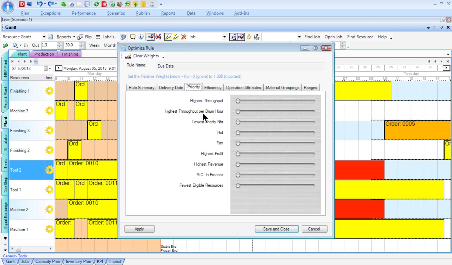
The financial KPIs are placed on the priority tab. If we wanted to, we could increase the weight assigned to the throughput tab so that the optimizer was adjusted to weigh throughput more heavily. Another option is to increase the weight placed upon the Highest Throughput per Drum Hour. Galaxy APS follows the Drum-Buffer-Rope optimization methodology. This is covered in Superplant. The drum is the constrained resource. Putting the throughput maximization on the drum/constrained resource makes the constrained resource one of the optimizer points.
The sliders can be changed in any number of ways. However, after all of the sliders are adjusted, one can see exactly the weights by selecting the Rule Summary tab.
One can go back and forth between the slider/adjustment rule screen, making changes, and then note how the KPIs change in this view. Furthermore, because there is a long list of data points held by Galaxy APS, one can compare the data points. This is not all that common in planning applications; much more work must be performed in other applications to pull off a simulation. The more difficult it is to perform simulations, the less they will be performed. The fewer simulations are performed, the harder it is for the company to determine the changes they should make to the system’s master data and configuration.
The History of Supply Chain Planning Simulation
During the software selection process, most companies don’t get into much detail on simulation. Companies ask for it, the vendors say the application can do it, and the box is checked; everyone moves on. When advanced planning was first developed, the simulation was supposed to be a big part of it. That projection did not come to pass. But without simulation, it’s difficult to know how to improve the settings in the system. Because of this, a lot of simulation functionality is half-baked. And as a result (along with a few other reasons), few companies have experience with doing a proper and structured simulation.
Simulation in Tabs in Galaxy APS
Galaxy APS has very user-friendly and low maintenance simulation capabilities. Galaxy APS is one of the few planning systems I am familiar with that keeps simulation versions — essentially a copy — in tabs. Each tab is a slight deviation from the other tabs,[5] allowing planners to switch very quickly between versions. With systems like SAP APO, creating simulation versions is a major effort, requiring planning and a good deal of time to copy the versions. I have spent quite some time creating functional designs that explain how APO simulation versions should be managed, their implications, etc. However, in Galaxy APS, simulation is seamlessly integrated into the standard user interface and does not seem to impose the massive overhead with APO planning versions. (I recently had to write up an entirely functional design for a client as to how a simulation version in APO would work that would support long-range planning and how it would be integrated into SAP BW. It was eventually postponed because of the amount of work involved.) With Galaxy APS, a planner can create a simulation version, make a few changes, run the optimizer, and if they like the output better than the version they copied from, they can only delete the first version. The “What If” scenario — represented by a tab —then becomes the live version. It is not a problem for the planner to keep open four or five tabs of different simulation versions. Hopefully, how easy this is to do is apparent.
In the book “Supply Planning with MRP, DRP, and APS Software,” I provide coverage to multi-objective optimization. Multi-objective optimization is still only rarely used for supply chain planning. However, there may be a role for it as the limitations of cost optimization and the issues with setting penalty costs are increasingly apparent. Details on this topic from several angles can be read at the link.
Multi-Objective and Goal Programming
Multi-objective optimization grew out of goal programming, something that people who have studied optimization are generally familiar with. Cliff Ragsdale makes the following point about goal programming in his excellent book Spreadsheet Modeling & Decision Analysis:
“The optimization techniques presented in the preceding chapters have always assumed that the constraints in the model are hard constraints, or constraints that cannot be violated. For example, labor constraints indicated that the amount of labor used to produce a variety of products could not exceed some fixed amount such as 1,566 hours). As another example, monetary constraints indicated that the amount of money invested in a number of projects could not exceed some budgeted amount (such as $850,000). Hard constraints are appropriate in many situations; however, these constraints might be too restrictive in other situations. For example, when you buy a new car, you probably have in mind a maximum purchase price that you do not want to exceed. We might call this your goal. However, you will probably find a way to spend more than this amount if it is impossible to acquire the car you really want for your goal amount. – Cliff Ragsdale
Goal Programming Problems
So, the goal you have in mind is not a hard constraint that cannot be violated. We might view it more accurately as a soft constraint representing a target you would like to achieve. Numerous managerial decision-making problems can be modeled more accurately using goals rather than hard constraints. Often, such problems do not have one explicit objective function to be maximized or minimized over a constraint set but, instead, can be stated as a collection of goals that might also include hard constraints. These types of problems are known as goal programming (GP) problems. Some additional comments should be made before we leave the topic of GP First, it is important to note that different GP solutions cannot be compared simply on the basis of their optimal objective function values. The user changes the weights in the objective functions from iteration to iteration; therefore, comparing their values is not appropriate because they measure different things. The objective function in a GP problem serves more of a mechanical purpose, allowing us to explore possible solutions. Thus, we should compare the solutions that are produced—not the objective function values. Second, in some GP problems, one or more goals might be viewed as being infinitely more important than the other goals. In this case, we could assign arbitrarily large weights to deviations from these goals to ensure that undesirable deviations from them never occur. lis is sometimes referred to as preemptive GP because certain goals preempt others in order of importance. If the target values for these goals can be achieved, the use of preemptive weights effectively makes these goals hard constraints that should never be violated.” – Cliff Ragsdale
Multi-Objective Versus Goal Programming
Multi-objective and goal programming both work and are most useful when the goals conflict with one another. This is undoubtedly true in supply planning, where service level being maximized directly conflicts with inventories being minimized. As pointed out by George Plossl:
“Efficient plant operation can be maintained if production levels are seldom changed, no overtime is incurred and machines are run for long periods once they are set up on a particular product; however, this results in large inventories and poor customer service while meeting the objective of maximum plant efficiency. Inventories can be kept low if customers are made to wait and if the plant is forced to react rapidly to changes in customer requirements and interruptions in production. In the business world, few companies can afford to work toward one of these objectives to the exclusion of the others, since all are about equally important for sustained success.” –George Plossl
Behaving Schizophrenically Regarding Objectives
While companies do generally behave schizophrenically when it comes to objectives (with objectives rising and falling in importance over time), the problem with cost optimization is that cost optimization is a single objective. Inventory optimization and multi-echelon (MEIO) planning are also more nuanced because it meets service level while minimizing inventories. However, this is not multi-objective optimization but is accomplished simply by setting the service levels as a constraint and then the objective function of reducing inventories. MEIO can also be run in reverse with the inventory as the constraint and the service level as the objective function (max). This can also be performed at many aggregation levels (for instance, service level in some MEIO vendors can be set at the customer of the contract — i.e., the equipment supported by the service level agreement.)
What is Pareto Optimality?
The concept of Pareto optimality was developed for situations for which there is not necessarily a global optimal developed, but the solution selected has no other better solution.
“A simple approach to solve such problems (MOO) is to express all objectives in terms of a common measure of goodness leading to the problem how to compare different objectives on a common scale. Basically, one can distinguish two cases. Either the search is for Pareto optimal solutions, or the problem as to be solved for every objective function separately.” – Real Optimization in SAP APO
One is a mixing approach, the Pareto optimal approach while selecting alternative optimal approaches. If the Pareto optimal approach is selected, some weighing is necessary for each objective function. The optimizer must be told the relative importance of each objective function in the global optimum.
Understanding Multi-Objective Optimization
Multi-objective optimization is actually easier to understand in my view than goal programming. Instead of one objective function being set up, more than one is set up. For instance, if you wanted to solve for two objective functions selecting between the speed of a transportation method and the cost of a transportation method, you would setup both objective functions in the problem and then solve for each separately, and then see the difference in what the optimization resulted in. This is implemented by using adding MINMAX constraints, which minimize the maximum deviation from the individual goals.
Conclusion
Many companies have sophisticated scheduling needs. Up until recently, these needs have been beyond the ability of most scheduling systems. Part of this reason is that the large ERP vendors don’t put much development effort into scheduling, and the smaller vendors have not created a compelling solution. This has recently changed. The SAP provides an integrated solution with PP/DS. However, the most effective approach is to use SAP planning modules for basic requirements but choose a best-of-breed solution for difficult or advanced requirements.
If a company implements any one of the three superplant functionalities, it will receive a financial benefit. superplant functionalities improve the company’s ability to leverage its resources and its suppliers, and its subcontractors. However, depending upon the application, financial measures can also be included in the optimization, which provides a direct linkage between KPIs and how the application makes decisions. In this way, financial considerations are both an input and output of a superplant.
Multi-objective optimization is intriguing, but it comes with its own implementation problems. One is that multi-objective optimization is more difficult to run because the individual options must be evaluated.
The other solution is the Pareto optimal approach, where weights are applied to the different objective functions. In this way, you tell the model which objective function should receive which emphasis during the run. I have found it very appealing one method is a single objective optimization, but with an adjusting heuristic, which allows for different objective weights to be applied to the optimizer. This is demonstrated in PlanetTogether, and which can be read about in this link.
[1] Apple Dictionary
[2] There are considered to have been two industrial revolutions. The first incorporated fossil fuel power generation, located within the factory, to drive a line shaft, which powered all of the factory’s machinery. The second was marked by electrification and the use of electrical motors in factories called unit drive. Many other inventions were part of the first and second industrial revolutions, but I have lumped both industrial revolutions into simply “the Industrial Revolution,” with a period spanning both.
[3] Optimization had been incorporated in customized solutions for quite some time before then, but I am referring to generally available off-the-shelf applications.
[4] Various financial KPI options can be used to adjust and drive the optimizer. I only want to cover a few in this book because all of the details of using financial KPIs to drive production planning and scheduling could be its book. One might look at these screenshots and ask the following.
“What is the difference between using the adjustment rule for Highest Throughput versus using the adjustment rule for Highest Profit?”
The difference is that in Galaxy APS, throughput subtracts the material cost for each order but no other costs. The Highest Profit adjustment rule, on the other hand, includes the comprehensive cost subtracted from throughput. This is just one example, but the Galaxy APS financial KPI adjustment rules can be used to provide an exceptional level of detail on the control of how the financial measures drive the optimizer. Furthermore, while I have kept this example simple for ease of explanation, any number of adjustment rules can be used per optimization run. This partially addresses one of the common problems with optimization projects, as described in the following article. https://www.brightworkresearch.com/sapplanning/2013/08/26/controlling-stock-pulling-location-optimizer/
[5] Galaxy APS takes advantage of multiple processors by assigning different versions — such as a simulation version — to different processors. Today, most servers that are sold have at least four processors. However, addressing each processor has proved challenging for supply chain planning vendors because a problem must be divided and then recombined as if a single thread processed it. However, Galaxy APS uses versions such that if a simulation version were to be planned, it would be assigned to an unused processor. In this way, it would not affect the system’s users as the production or live version of Galaxy APS is on a different processor. This is a differentiator regarding how expensive it will be to provide hardware for the application. An application with a limited ability to leverage the other server processors will need to purchase a significantly more expensive server. I recognized this when analyzing Galaxy APS: its hardware requirements were deficient compared to other applications with which I was familiar. Secondly, utilizing multiprocessors means that the application can also leverage servers with even more than four processors, opening up more opportunities to buy good-value hardware.
[6] As I have alluded to several times, both APO and Galaxy APS “have” simulation capabilities. However, just because they both “have” functionality says nothing about how superior one is to the other. Because executives don’t create simulation versions or otherwise use the applications they purchase, it’s easy to lose the shades of gray and homogenize the functionality between two vendors. Furthermore, a skilled presales consultant with a canned demo, who trains the application, can make very difficult-to-use functionality look quite easy to master.
References
“Spreadsheet Modeling & Decision Analysis: A Practical Introduction to Management Science, 6th Edition,” Cliff Ragsdale, South-Western, 2010
“Production and Inventory Control: Techniques and Principles 2nd Edition,” George Plossl, Prentice Hall, 1985
“The Future of Everything: The Science of Prediction,” Dr. David Orrell, Basic Books, 2006
https://en.wikipedia.org/wiki/Minimax
“Optimization Modeling and Spreadsheets,” Kenneth R. Baker, Wiley, 2011 “Real Optimization with SAP APO, “Josef Kallrath, Thomas I. Maindl, Springer Press, 2006