How to Best Set Up the SAP SNP Optimizer

Executive Summary

• The SNP optimizer is the CPLEX optimizer now owned by IBM.
• We cover how to use a heuristic with the optimizer and comparative optimizer settings, costs, ordinary optimizer, and problem segmentation problems.

Introduction: Getting into Depth on the SNP Optimizer

The SNP optimizer has many essential features not published due to those that write on the optimizer being aligned with SAP. You will learn what are frequently hidden SNP optimizer topics.

What is the SNP Optimizer?

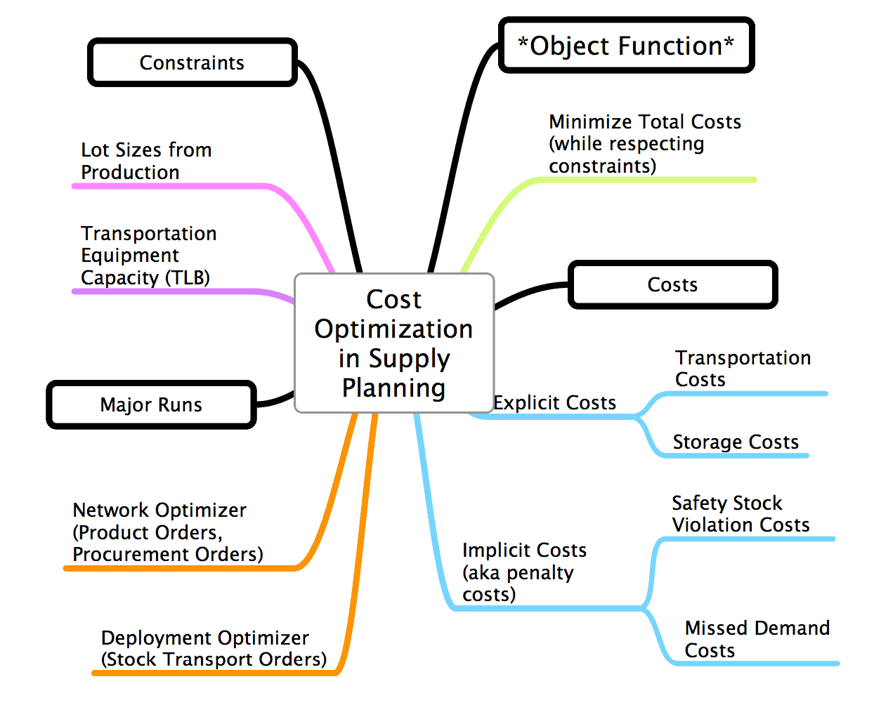
The SNP Optimizer is one of the three supply planning methods available within SNP (the others being CTM and heuristics). The SNP Optimizer uses an objective function which is to minimize costs (or the very maximize profit) subject to constraints, and driven off of costs which are the following:

1. Unfulfilled Demand Costs
2. Production Costs
3. Safety Stock Costs
4. Storage Costs
5. Transportation Costs
6. Shelf Life Costs

The SNP Optimizer attempts to manage all these costs by making decisions (such as creating purchase requisitions, production requisitions, or stock transport requisitions), which minimize the total costs. The costs are composed of “explicit” and “implicit” costs.

The CPLEX Software that Runs the SNP Optimizer

The SNP Optimizer is made up of three major components:

1. The optimization engine (provided by CPLEX)
2. The optimization mathematics (provided by SAP and which are proprietary but based on public research and not much different from other supply planning cost optimizers)
3. The optimization master data (the costs and the optimizer profiles, etc.)

This quote provides some more detail about the CPLEX engine.

“The SNP optimizer in SAP APO is based on linear and mixed integer linear programming (LP and MILP) using ILOGs CPLEX, the optimization engine. LP problems can be solved with the primal simplex, and the dual simplex or interior point methods. The decision about the sources for the products in question depend upon the results costs.” – Real Optimization with SAP APO

About CPLEX, ILOG, and IBM

ILOG CPLEX is the optimization engine for many enterprise applications in the supply chain space, and more about it can be found on the ILOG CPLEX page. SAP simply creates an input user interface and then configuration settings that control the weights of the costs that go into ILOG CPLEX.

ILOG CPLEX uses costs to perform the optimization.

• ILOG CPLEX was created by what was once an independent company called ILOG.
• After CPLEX was added as the optimizer to APO, ILOG was purchased by IBM.
• Because IBM increases the software price that it acquires but essentially stops developing it, CPLEX is no longer a desirable product. It is now no longer considered competitive with other optimizers on the market.

SAP likes to keep it quiet that the optimizer in APO is not its creation but is, in fact, ILOG CPLEX. It is prevalent to arrive at SAP customers who have never heard of ILOG CPLEX and thought SAP created their optimizer. Therefore, the output is the ILOG CPLEX optimization.

• This shows the inputs and the controls for the SNP optimizer. This applies to both the network and the deployment optimizer runs in SNP.
• This graphic will help anyone understand all the inputs to the optimizer. What costs can be set, etc..
• However, how the costs are set is another detailed topic.

Optimization Profiles

Profiles control the SNP optimizer. 97 parameters are distributed across seven tabs. They provide a very high level of control over how the optimizer operates. This allows the parameters to be assigned to product locations. This is very similar to the configurations set up on the Deployment Optimizer side. However, there are some field differences.

The deployment optimizer has an extra tab specifically for deployment. The deployment optimizer profile is covered in this article.

The setup of this profile can be found by looking under…

APO – Supply Network Planning – Environment – Current Settings – and then profile and then Define SNP Optimizer Profiles

 

Or it can be found in SPRO here.

You will want to create a new profile by naming it and providing a description.

This brings up the configuration area.

The first decision to make is whether SNP should perform linear or discrete optimization. Discrete optimization is recommended for the final plan as it is more realistic and considers things like lot size.  You must define which you want SCM to take into account.

I quote from SAP Help below:

The General Constraints Tab

“On the General Constraints tab page, first activate the constraints that you want the optimizer to consider independently from the chosen optimization methods, such as production capacity, storage capacity, and transportation capacity, or take the minimum PPM lot size or minimum transport lot size into account. On this tab page, also define whether you want the optimizer to take into account the safety stock. If you do, you can specify whether you want deviations from the safety stock to be taken into account as an absolute value or as a percentage during the penalty cost calculation. You are also able to define whether you want the optimizer to take into account the shelf life of products and if so, whether you want to continue using the product after it has expired (passed its shelf life expiration date) or whether you want to dispose of the product. If you want to continue using the product after its expiration date, you are also able to define whether you want the optimizer to use the procurement costs that have been defined for the location product (default setting) as penalty costs or whether you want it to use penalty costs that are not product-dependent (if you wish to use this option, enter an appropriate value).” – SAP Help

The Discrete Constraints Tab

“If required, on the Discrete Constraints tab page, activate constraints that you want the optimizer to take into account for the discrete optimization method, such as integral (integer value) or minimum lot sizes for transportation or the production process model (PPM). A prerequisite for being able to make settings on this tab page, is that you have chosen the Discrete Optimization method in the header data.”

SNP can be run with just one constraint or all the restrictions listed, providing very significant flexibility.

“Constraints considered by the SNP Optimizer can be soft, pseudo-hard, or hard. Examples for soft constraints are bottlenecks which are caused by delivery dates and that can be compensated by capacity expansions or additional shifts. Soft constraints can be “violated” by the solution resulting in penalty costs that go in the objective function. Pseudo-hard constraints are characterized by possible violations that, however, result in very large penalty costs.” – Real Optimization with SAP APO

The Model Parameters Tab

The Solution Methods Tab

The Solutions Methods tab is where the critical maximum runtime is set. Cost optimizers are given windows of time within which they must come to a solution. This window’s determination should be based upon the operational workflow between systems—coming to a correct window. This is important because optimization tends to run longer than the operational workflow (the time available for system processing and the sending and receiving of data between systems) will allow. Capping the time can often bring good solutions, and allowing the optimizer to continue running after a certain point often does not lead to a better solution. However, to find this point, iterative testing at different durations must be performed.

This is accomplished by running the optimizer for varying amounts of time and showing the results to planners to find the optimizer’s point of diminishing marginal utility or benefit of the results.

If the runtime is too large to achieve the optimal business benefit, then changes can be made to the optimizer model or extra hardware, and things like parallel processing profiles can be set up (advisable regardless) to help reduce the optimizer runtime.

This is discussed in more detail in this article:

The decomposition options, which is how the problem is broken down, are covered in-depth in this article.

Solution Procedures

One of the most important selections is the solution procedure that is selected. This is another complicated subject that is better covered with its post.

The Integration Tab

On the Integration tab page, define parameters for integrating SNP optimization and Production Planning and Detailed Scheduling (PP/DS). You can specify that you want the optimizer to consider the production horizon and the stock transfer horizon and whether you want the optimizer to consider dependent demand and distribution demand resulting from fixed orders as a hard constraint or a soft constraint. Soft regulations can be violated with resulting penalty costs.

You can also choose whether you want the optimizer to consider the stock of PPM input products or source location products that have not been selected. Within-lot size planning, you can also specify whether you want the optimizer to take into account the setup statuses planned in PP/DS. – SAP Help

The Extended Settings Tab

“On the Extended Settings tab page, specify the type of consistency check (if any) you want the system to make and whether you want the log data for an optimization run to be stored. On this tab page, you can also specify that you want the optimizer to ignore the time-based constraints you defined in interactive planning. You can define whether you want the optimizer to take the time-based upper bound for stock as a soft constraint or a pseudo-hard constraint; which means, whether they can be violated with incurring penalty costs. You can also define how you want the optimizer to proceed if it cannot find a solution for a problem within the specified runtime. First, you can enter a runtime extension. If the optimizer cannot find a solution by the end of the extended runtime, other options are available (such as, simplification of the problem).” – SAP Help

The Automatic Cost Generation Tab

It is well known that costs must be generated for the optimizer to make its decisions. However, SNP Optimizer offers automatic cost generation.

“On the Automatic Cost Generation tab page, define the business goals based on which the optimizer generates all the relevant control costs. If you want to use the automatic cost generation function, you have to set the corresponding indicator in the header data of the transaction.” – SAP Help

“You are also able to define whether you want the optimizer to take into account the shelf life of products and if so, whether you want to continue using the product after it has expired (passed its shelf life expiration date) or whether you want to dispose of the product. If you want to continue using the product after its expiration date, you are also able to define whether you want the optimizer to use the procurement costs that have been defined for the location product (default setting) as penalty costs or whether you want it to use penalty costs that are not product-dependent (if you wish to use this option, enter an appropriate value).” – SAP Help

This is hypothetically how shelf life would work. I have yet to see shelf life functionality work in SNP. However, shelf life costs are calculated during an optimization run. Issues with shelf life are described in this article.

Using the SNP Optimizer with a Heuristic

The SNP optimizer an option called the Heuristic First Solution. This is shown in the screenshot below.

How Optimization Problem Solving Works

Optimization is usually presented as mathematically pure. However, the truth is that optimization often requires a lot of help to perform effective problem solving. One form of support is called decomposition, which is the dimension under which the problem is segmented into small issues to reduce the solution space. One way to do this is to divide by product so that only part of the supply chain network is being processed at one time.

The solution space is where the optimizer needs to look for the best solution to find its answer. The smaller the solution space can be made before the optimizer begins its work, the better it will be at problem-solving. Solution space bounding is one of the best ways to improve the optimization results.

This setting is a second way of helping the optimizer. This is, in fact, very similar to simulated annealing. Wikipedia’s definition of simulated annealing is listed below:

“Simulated annealing (SA) is a generic probabilistic metaheuristic for the global optimization problem of locating a good approximation to the global optimum of a given function in a large search space. It is often used when the search space is discrete (e.g., all tours that visit a given set of cities). For certain problems, simulated annealing may be more efficient than exhaustive enumeration — provided that the goal is merely to find an acceptably good solution in a fixed amount of time, rather than the best possible solution.” -Wikipedia

What The Heuristic First Solution is Similar to in Other Optimization Applications or Approaches in Supply Chain Planning

By the way, for those that might be wondering, “exhaustive enumeration” is allowing the optimizer to run and to “enumerate” all of the different options before selecting one. However, while the Heuristic First Solution is similar to simulated annealing, there is an important difference. Simulated annealing is itself a non-optimization method for problem solving. The Heuristic First Solution starts by applying a heuristic to find the right “neighborhood” and then uses the optimizer to search within the neighborhood.

Therefore in some cases, the best first move that a supply chain network optimizer can make is to get assistance for problem-solving. This would be a little like a GPS asking for directions to a city before performing the calculation to get to a particular address. GPS, of course, doesn’t have to do this because the problem they are solving computationally is much more straightforward. So simple that it can be solved in most often less than a minute (unless long distances are required to be calculated) by the low-powered processor that resides within most GPS units.

Other Applications

Other linear programming-based optimizers have this same type of functionality. Typically, running LP on an empty solution space is quite time-consuming. Two approaches, for instance, which are available supply chain planning applications that include i2’ s/JDA’s SCP, are the following:

1. Store the result in binary mode (memory map so sort) and then use it as the next run’s initial point.
2. Make some heuristic approximation to get an initial point. <– this will be mostly discrete by the vendor. Even in i2, there were various ways of doing this cross-product line/solution.

So SAP has it (although it is very lightly documented), and i2’s SCP optimizer has the setting as well. Another vendor has it as well. This should not be surprising as both i2 and SAP’s solver is CPLEX, so obviously, the applications only make the options available within the application reflective of the same (although much more limited) switches available in the CPLEX solver.

However, the question remains as to how to use the setting. Typically instructions are required to “form” the heuristic before its use. Yet, I have not found instructions on how to use this setting in any online documentation. Of course, the setting could simply be tested by turning it on before an optimization run, but of course, this would need to be performed in a simulation environment.

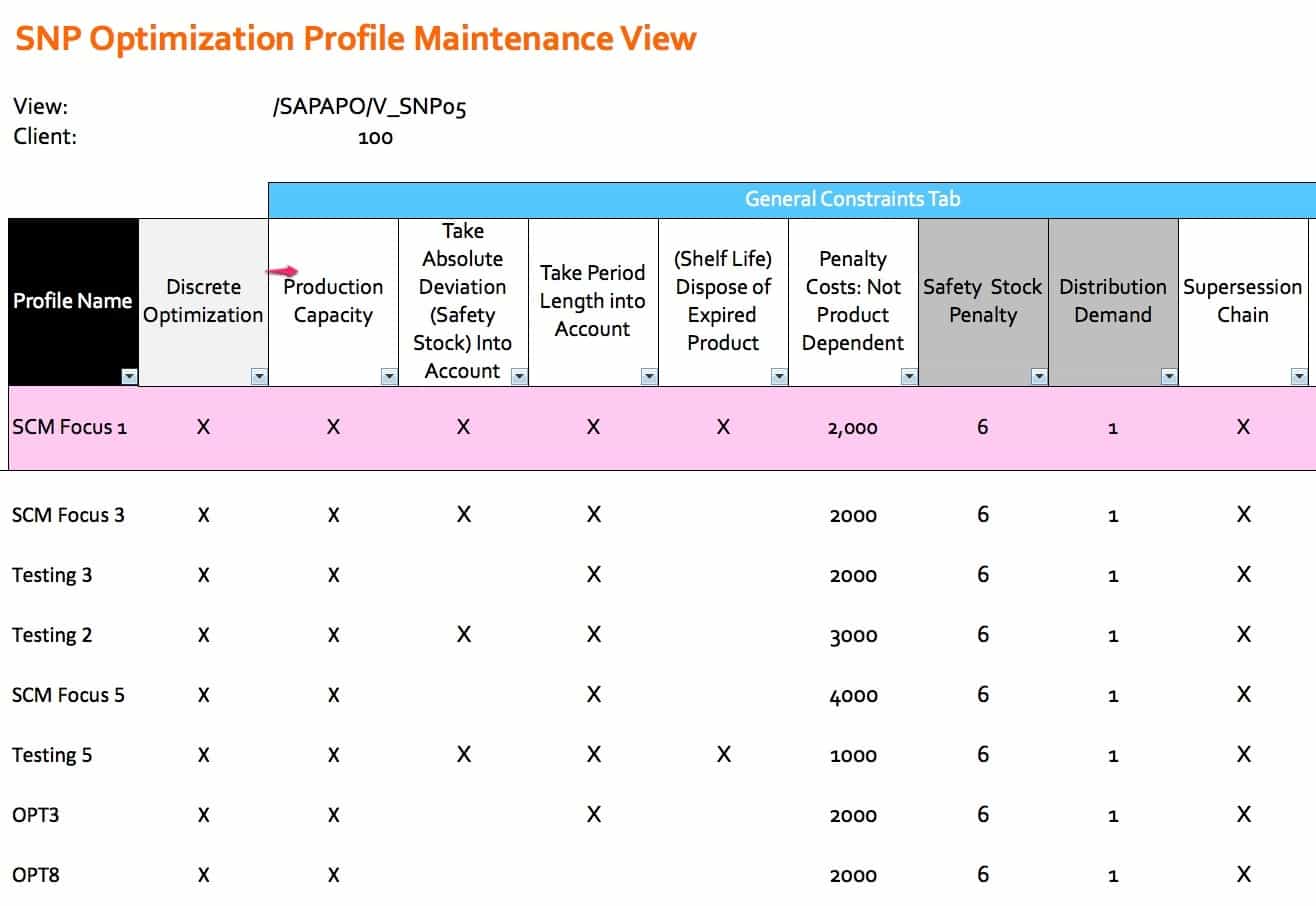
Comparative Optimizer Settings

This shows the settings of an SNP optimizer regarding how its different profiles compare to one another. This was taken from an actual project. Only the profiles names have been changed. The settings are exactly as were used in an operating SNP system.

Optimization Segmentation Problems

Optimization problems are important to divide into smaller problems. The less the solution space can be made to be, the more efficiently the optimizer will solve it. This is a type of decomposition, as decomposition is often considered to be performed by the solution itself. For instance, the SAP SNP Optimizer can decompose its problem based upon product, resource, or time. The type of decomposition I am referring to is the manual type, where the overall model is divided into runs.

The trick in problem Division is to split the problem so that the interrelationships in the model are all in the same run. For instance, if a location is to supply another location, those two locations must both be in the run. Companies often have many interdependencies they want the optimizer to solve for. Often the way that optimization runs division is somewhat arbitrary. It does not have to be. Optimization can be used to develop an optimum problem division.

The Problem Type

Optimization has many different types of problems that it can solve. The problem that is being solved is the most critical factor controlling how the problem is set up. A well-known optimization problem is a traveling salesman problem. In this type of problem, the distance is minimized through a series of required steps. Supply planning problems are the network flow optimization type where material must flow through a network of nodes, which have different constraints.

Segmentation Problems

The classification of the problem, which applies to any attempt to divide list items into different segments to meet some objective, is called segmentation problems. Because the problem is often based on various criteria, the problem may also be referred to more specifically as the multi-criteria segmentation problem. In this type of problem, the straight line distance is created for each criterion, and the distance between each criterion is minimized within its grouping. Some interesting notes on segmentation:

“Now suppose, instead, that we are allowed to create two catalogs each with r items, sending one of the two to each consumer; obviously, there are cases in which the value we obtain from a pair of catalogs cangreatly exceed the value obtainable from one.

Segmentation problems address the problem of the degree of aggregation in the data that an enterpriseuses for decision-making. Any enterprise faces an optimization problem”

These are maximization problems. Thus the objective function is to maximize the number of divisions but given specific constraints. These problems can also be set to make the number of segments a particular number.

“For example, mail-order companies produce several hundred different catalogs each year, targeting one or more at each of the customers on their mailing list. A telephone company may divide its customers into two segments: residence and business customers; they offer different terms and prices to the two. How can such segmentation decisions be arrived at in a principled and automatic manner? In each situation, what is the optimal level of aggregation, and what is the corresponding optimum ensemble of decisions? Segmentation problems, as defined and studied in this paper, are stylized computational problems whose intention is to capture these important question

Note the apparent similarity between segmentation problems and facility location problems, in which one must open” some number of facilities to serve customers: there is a cost for each facility opened, and apenalty for each customer-facility distance. The issues in our algorithms here turn out to be technically quitedistinct from those in facility location problems. First, the problems we consider here center around maxi-mization rather than minimization, and this changes the nature of the approximation questions completely.Moreover, our space of possible decisions is typically exponential or innite, and only implicitly represented”

Background on Costs in the Cost Optimizer

Recently I have been reviewing the cost settings of several clients. One of which was interesting and this type of review is something I recommend for all cost optimization projects. With this client, it turns out that the costs for the different categories were set up in this proportion.

1. Transportation Costs = 1 to 3 (depending upon the mode)
2. Storage Costs = 100 to 140 (depending upon the location product combination)
3. Unmet Demand Costs = 75,000 to 95,000 (depending upon the location product combination)
4. Safety Stock Violation Costs = 200 to 350 (also depending upon the location product combination)
5. Manufacturing Costs 1 to 4 (depending upon the product line combination)

What These Costs Mean

At account at after account, the management at these companies questions what the optimizer is doing. It is not only the management; often, the configurations have similar questions. They are often so busy with other activities that they do not have time to evaluate the costs that are driving the optimizer. Often costs optimizers are referred to as “black boxes” by people surrounding the implementation at companies. While fully understanding optimization mathematics may be complex, what cost optimizers are doing is not complex. The objective function says it all, minimize costs. The strength of all forms of optimization is that they can balance some factors all at once. The cost optimizer built into SNP (which is CPLEX incidentally, SAP purchased the CPLEX solver which resides inside of SNP, PP/DS, and TP/VS) can look at all the costs listed above. It is not only trading off these costs for a single product along the lines of

• Transportation costs
• Storage costs etc…

It is s also trading off all the costs in all the categories for all the products versus one another. This is a big “however,” it can only do this if the costs are set up in a way that allows this to happen. The costs you see listed above do not let this happen. No overall optimization is going on because the costs of unmet demand are so high that they dominate all other system costs.

The instruction to the optimizer is simple.

“Meet demand no matter what the costs.”

The Problems with Setting Costs This Way

This is the unintended consequence of setting a cost category so high about all the other costs. It removes the model’s flexibility to trade-off among the different costs and only allows two forms of optimization to occur. These are the following:

1. Costs within a cost category (therefore, lower costs can be set for transportation modes (such as a truck) that cost less than rail. This will cause the optimizer to choose rail to select the mode and still meet the demand date.
2. Costs between products. If a location only has enough capacity to manufacture Product A, which has an unmet demand cost of 95,000, or Product B, which has an unmet demand cost of 75,000, the optimizer will choose to produce and satisfy the demand for Product A.

Controlling the Stock Pulling Location with the Optimizer in SNP

This article responds to a question about the Brightwork Research & Analysis Press book Setting Up the Supply Network with SAP APO. The scenario is as follows:

I have a forthcoming piece of work looking at the use of SNP optimizer for purchased products. A typical scenario is:

• Forecast at DC A
• DC A can be serviced (for stock replenishment) from other DCs B and C, and also from vendors.
• We need to set the optimizer such that to meet forecast at A, we first use available stock from B and C, before requesting any further supply from vendors.

The Question Diagram

To best understand this question, it makes sense to diagram the problem, which I have done below.

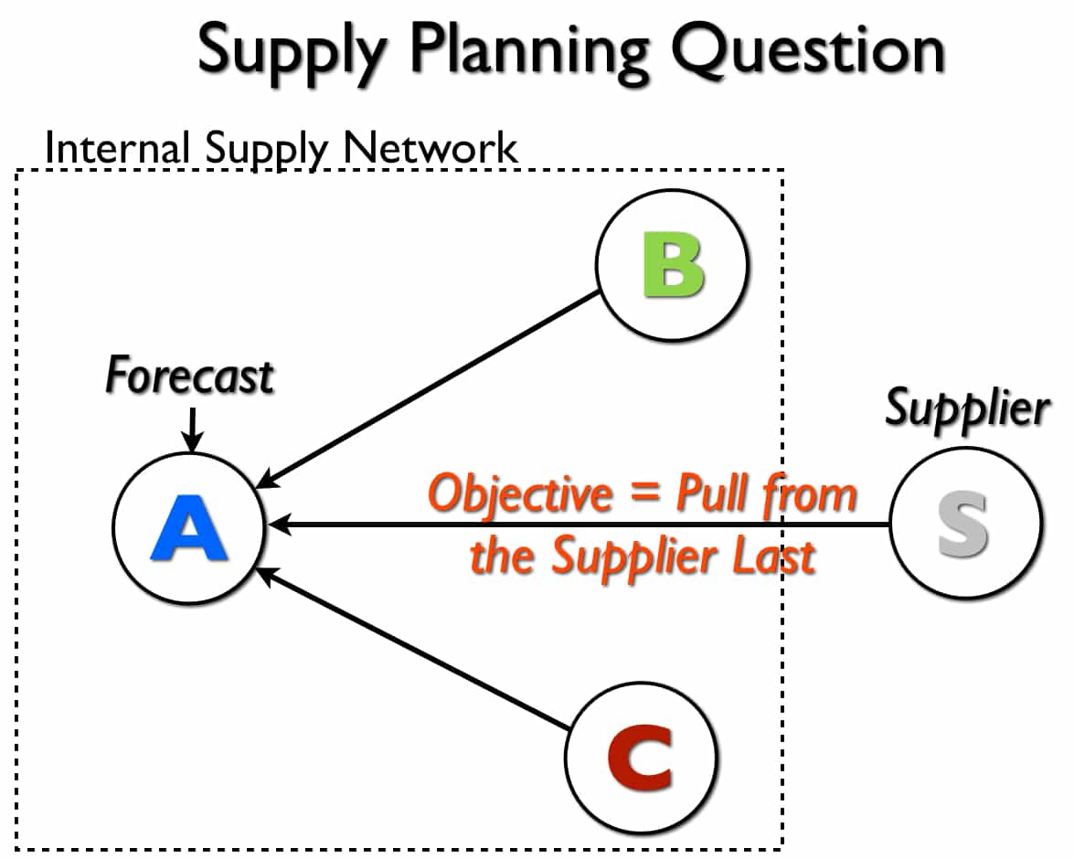
This shows that there are three sources of supply for location A — which is a location that receives the forecast. 

Different Approaches to Solve the Problem

There are quite a few ways to solve this problem — and several which I don’t recommend. SAP has spent time explaining that the SNP optimizer can be used along with priorities. I have never been satisfied with how the SNP optimizer performs decision-making, except when costs are used.

Within the category of costs, there are again several ways to solve this problem. One of the trickiest parts of setting up costs in the cost optimizer is agreeing to what costs will be used to control what desired outcome.

How Costs Tend to be Documented on APO Optimization Projects

I have written quite a bit about how costs are set in far too much an ad-hoc manner. Furthermore, it is difficult to find documentation at clients that explain what the intended result of costs is — merely a listing of the costs or the costs are an insufficient explanation of the mindset and methodology for cost setting. However, this incomplete approach is the dominant way to implementing cost optimizers — and this is not only restricted to the SNP or PP/DS optimizer. This is a serious problem that is partially responsible for optimizers adding so much less value than they were initially proposed to add when they were first introduced in the supply chain planning market.

The Answer Diagram

Below, I have set up — with all other costs being equal (PPM/Storage/etc…) costs being equal, this adjustment to the transportation lane’s costs will provide the desired outcome. However, as soon as the other costs differ, all bets are off.

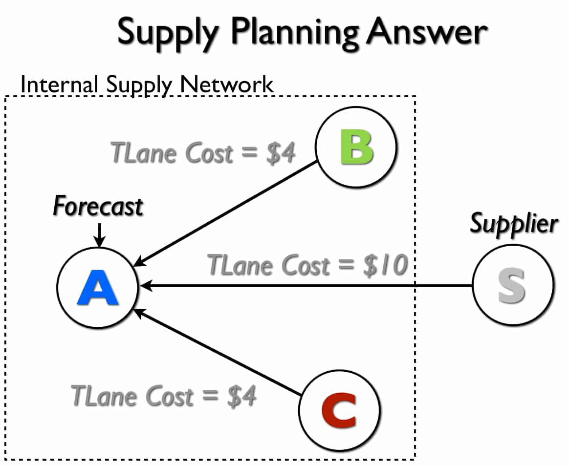
Because the SNP optimizer will incur more costs when it transports the product from the supplier versus Location B or Location C, the supplier should be the last place it pulls stock from. The optimizer will prefer to flush the stock from these two internal locations first because it costs less to do so. 

Caveat & Conclusion

The solution that I have provided to this question is misleading simply. Yes, one can solve any one problem with a specific set of costs — however one is never attempting to solve one problem. Instead, a range of behaviors is desired, and the costs set up to provide one behavior can adversely affect the other desired behaviors. And, of course, what the company wants to do tends to broaden over time, so small changes to the optimizer costs can lead to big problems as the previously set costs are often tinkered with as time passes.

This is the logic for testing any new adjusted cost in a simulation version where the entire model is the same, except for a single change made to a category of costs.

The Concept of Local Optimums

The condition of not being able to optimize the over system, but focusing on optimizing subsets of the overall problem, is called solving local optimums. I discuss global versus local optimums in this article.

What is highly interesting about this is that most companies that are setting up costs have no idea they are undermining their optimization software. To maximize service level, they are so tilting the playing field in the direction of one goal that they have greatly simplified, and not in a good way, the problem the optimizer has to solve.

Standard Models

SNP is software by SAP, and they really should be providing more thought leadership to clients, but I don’t find this. I have heard this same feedback from multiple clients. This is brought up also by the book Real Optimization with SAP APO.

“SAP’s in-house consultants will help explain the underlying mathematical assumptions, but consultants with deep optimization and business software knowledge are often scarce.” – Real Optimization with SAP APO

I have recently begun to question why SAP does not offer several standard cost models with its optimizers that have tended to work for different industries. This would be very easy for them to build as they have access to their client’s cost data. There is little reason for every company to re-create the wheel when it comes to optimizer costs.

Solving the Model

The book Optimization Modeling brings up an excellent point with Spreadsheets regarding what is being solved during optimization.

“Whether we have tactical information or strategic information in mind, we must still recognize that the optimization process finds a solution to the model, not necessarily to the actual problem. The distinction between model and problem derives from the fact that the model is by its very nature a simplification. Any features of the problem that were assumed away or ignored must be addressed once we have a solution to the model.” – Optimization Modeling with Spreadsheets

When is Cost Optimization a Good Choice for Supply Planning?

The operative word is “complicated,” that is, the supply planning problem that is to be solved should be complex.

Mathematical optimization is extremely useful if the underlying decision problem can be quantified and involves many degrees of freedom (each of a number of independently variable factors affecting the range of states in which a system may exist – Wikipedia) and constraints leading to a complexity which is not easy for human beings to grasp Ideally the kind of optimization we have in mind is best for reasonably complex production networks with utilization rates close to 100%. If the product network is utilized say up to 40%, then the decision of where to produce how much of a certain product is not too difficult. Mathematical optimization can do it but probably the human planner can do it as well. – Real Optimization with SAP APO

Major drivers towards cost optimization include the following:

1. The desire to perform multi-sourcing (multiple locations can supply a location)
2. The desire to perform constraint-based planning
3. The interest in having costs control the supply network (I have said that cost minimization previously is an important assumption, but because the costs used in cost optimizers have so little to do with actual costs, this assumption is not necessary to hold to use cost optimization)

The Complexity of Using the SAP APO Optimizer

Implementing and maintaining optimization methods requires much effort and long-term investment. Secondly, optimization requires a great deal of discipline and knowledge on the part of the implementing company. Many companies want the benefit of advanced planning but are not culturally, financially, or skills-wise prepared to make the sacrifices required to get the desired outcomes.

More often than not, companies want simple solutions that deliver value quickly. That isn’t how optimization works. And this is partly because the software has historically been designed to be more complicated than is necessary.

Stories from the Field with the Optimizer

There is a story about an advanced planning vendor running the optimizer engine in the background, but when the engine went down for a few days, no one even noticed. This was because the planning was primarily being performed by heuristics that had been custom coded with scripts, and the solution was not using the optimizer at all.

Whether the client knew the optimizer was not being used is unknown. This is more common than reading press releases, and industry periodicals in the area would make you think. While optimization sold a lot of supply chain software, it wasn’t necessarily what the customers went live with, as evidenced by this example.

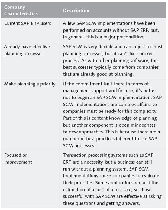
What Companies Are Right for the SAP APO Optimizer

Some companies are better suited to undertaking SAP APO optimization than others, and Table 1.1 shows the typical characteristics that allow a company to be successful with the optimizer.

One way of looking at whether your company is appropriate for SAP optimizer is to determine if it has maximized the planning functionality within SAP ERP. And in some cases, requirements will naturally lead to the consideration of SAP APO.

More generally, the APO optimizer is most beneficial to companies dedicated to improving their planning processes, and that already have good planning processes to begin with. This statement isn’t only true of the SAP APO optimizer but of advanced planning tools generally. While we’re not able to find specific research to back this up, our anecdotal evidence from our experience on projects indicates that the better the company is planning before it implements an advanced planning system, the more the company gets from the implementation. Effective planning helps the company know how to design the system and allows the company to better leverage what it ends up implementing.

Global Versus Local Optimums

Nonlinear optimization tends to be expressed as much more straightforward than it is. While linear optimization is straightforward, things become much more complex as soon as nonlinear constraints are added. This, of course, has to happen to model the realities of the supply network. As soon as lot size is added to the optimization, the optimization becomes nonlinear. While linear optimization will, in most cases, find the global optimum (although the constraints can still be wrong, and in fact, the objective function can be false as well), nonlinear optimization is not guaranteed to find the global optimum. It can get caught in a local optimum.

Nonlinear Optimization and Basins of Attraction

This is because while linear optimization has a single basin of attraction, nonlinear optimization can have any number of basins of attraction. If the solution gets caught in one of these non-global basins of attraction, then the result is a local optimum. This is a sticking point for explaining optimization to companies, but MathWorks online helps this well.

Generally, Optimization Toolbox solvers find a local optimum. (This local optimum can be a global optimum.) They find the optimum in the basin of attraction of the starting point.

There are some exceptions to this general rule.

• Linear programming and positive definite quadratic programming problems are convex, with convex feasible regions, so there is only one basin of attraction. Indeed, under certain choices of options, linprog ignores any user-supplied starting point, andquadprog does not require one, though supplying one can sometimes speed a minimization.
• Global Optimization Toolbox functions, such as simulannealbnd, attempt to search more than one basin of attraction. – MathWorks Help

Simulated annealing is a method of finding an optimal solution that uses a metaheuristic rather than “straight” optimization, which is also termed exhaustive enumeration. Techniques for helping the optimizer find the global “pretty good solution” become more critical as the problem becomes more complex and the solution search space becomes larger. The more I use optimization systems. The more critical these types of approaches seem to be.

With massive problems, pure or “straight” optimization takes too long and has too many complications. This can take some skill to explain to companies as optimization is often explained to them during the software selection phase as something which can produce a perfect solution.

Searching for a Smaller Minimum

If you need a global optimum, you must find an initial value for your solver in the basin of attraction of a global optimum.

Suggestions for ways to set initial values to search for a global optimum:

• Use a regular grid of initial points.
• Use random points drawn from a uniform distribution if your problem has all its coordinates bounded. Use points drawn from normal, exponential, or other random distributions if some components are unbounded. The less you know about the location of the global optimum, the more spread-out your random distribution should be. For example, normal distributions rarely sample more than three standard deviations away from their means, but a Cauchy distribution (density 1/(π(1 + x²))) makes hugely disparate samples.

Some people on a project may have had experience with linear programming/optimization, but fewer will have had experience in nonlinear optimization. While finding the global optimum is both straightforward and fast for linear programming, it is much less so for nonlinear. Of course, the majority of cases of supply chain optimization are both nonlinear and integer.

When Sub-Problems Solve Feasibly

A subproblem is based upon how the optimized has decomposed or segmented the problem. For cost optimization in supply planning, common decomposition methods are:

1. Location
2. Product
3. Resource
4. Time

The SAP SNP Optimizer shows several of the settings above in its optimizer profile in the screenshot below.

Probably the most common, however, is decomposition by-product. However, multiple types of decomposition can be combined. Using decomposition by-product divides the overall supply network into a series of sub-networks based upon the product groups. Therefore if products A, B, and C are stocked in locations 1, 3, 5, and 8, only these locations are analyzed for that particular sub-problem.

When the Optimizer Takes Too Long to Finish and Times Out

There are two basic states for any sub-problem at the end of an optimizer run, either optimally solved or feasible. All solutions will be feasible; therefore, it is axiomatic that a subproblem that does not solve optimally will solve feasibly. As we discussed earlier, just because a nonlinear problem solves optimally does not mean that it found the global optimum. Secondly, when a subproblem returns a feasibly solved, it is tough to determine how far away the found solution is the optimal solution. For instance, with one very well-known cost optimizer for supply planning that I use, there is no quantitative information about how far the solution is from the optimal. When problems surface in the supply plan, it is the case that infrequently, the sub-problem associated with the product has not been solved optimally.

How far is the proposed solution from the optimum? Most enterprise optimizers do not provide the diagnostics to find out. This leads to the next point.

Proper Sizing of the Hardware For the Optimizer Based Upon the Percent Optimally Solved

Nonlinear optimization firstly takes quite a bit longer to solve than linear optimization. This is the main reason that often linear optimization is run to reduce the solution space. Some optimizers apply the same linear optimization determined solution space every time before nonlinear optimization is run or only periodically change the linear optimization determined solution space when something is changed.

Secondly, because many enterprise nonlinear optimization applications do not have metrics for how far feasible solutions are optimal, it can make hardware sizing problematic. Some vendors provide good metrics on optimizer sizing, by others do not. Optimization sizing is tricky because how long an optimizer will run is based upon a variety of factors, some of which are listed below:

1. The volume of transactions
2. The size of the supply network
3. The number of constraints
4. How the problem is decomposed
5. How the costs in the system are set up relative to one another
6. What other ways the optimization problem is divided (decomposition is segmentation performed in the optimizer; however, there is any number of ways of dividing the problem so that there can be separate runs. For instance, a company can use the product decomposition setting within the optimize, but segment the runs by those products that run on particular resources, so in this way, it can achieve both internal product decomposition and external or manual resource decomposition)

Parallel Processing Profiles

Specific technical configurations can be set up, such as parallel processing, which can significantly speed calculation time. Parallel processing is a method of maximizing the CPUs’ use by allowing the server’s processor to be fed the problems in multiple streams rather than as a single stream. As it is now common to have multiple CPUs in a server, this is a method of adjusting the software to match the hardware that many businesses already have. To compare run times between the methods, similar parallel processing profiles must be set up for each process for the rough benchmarks I provided to apply.

Model Simplification

There are additional ways to speed the processing within any one method, which typically involves either reducing the model’s complexity (for instance, the number of valid location-to-location combinations) or by dividing the problem into smaller pieces. However, as hardware becomes more powerful and less expensive every year, techniques necessary to increase runtime in the past are not necessarily applicable now. The best example of this is found in demand planning, where techniques that were used for increasing the speed of forming attribute relationships are now no longer necessary.

Reducing Absolute Optimality

While achieving an optimal solution is the desired end state, practical considerations often get in the way of this goal. Therefore to get to “still good” solutions but within time and hardware budget constraints, one method employed is to reduce the level that the optimizer must achieve before it completes its search/calculation. The following quote explains this well:

“The optimizer does not always solve integer programs to optimality. The tolerance parameter in the Solver Options dialog box is set to 5% by default. This means that the optimizer will stop when the solution is within 5% of the true optimal solution. Even with the tolerance parameter set to 5% the optimizer will often give the true optimal solution. The default setting is .05 because integer programs can take a very long time solve. To ensure that the exact optimal solution is obtained, the tolerance parameter should be set to 0.0%”– An Introduction to Spreadsheet Optimization Using the Excel Solver

How to Use the SNP Optimizer Log for Analysis

This document is designed to explain how to use the SNP optimizer log to analyze the system. The SNP optimizer has a log, which provides information on various things, which can be useful in understanding the system’s output and troubleshooting the system. The log can be read within SAP or can be exported as a flat-file. There are benefits to using the log in each way. The log can be read within SAP to find information quickly, and the export of the log in the form of a log trace file can be performed to keep an archive of each optimizer log run.

The logs kept in SAP are gradually deleted as time passes, and currently, only two weeks of previous logs are held in the system. However, by exporting the log trace file, an unlimited number of logs can be kept and compared.

Getting to the Log

The log can be obtained by going to the transaction /N/SAPAPO/SNPOLOG.

After you type in this transaction, the following screen will come up.

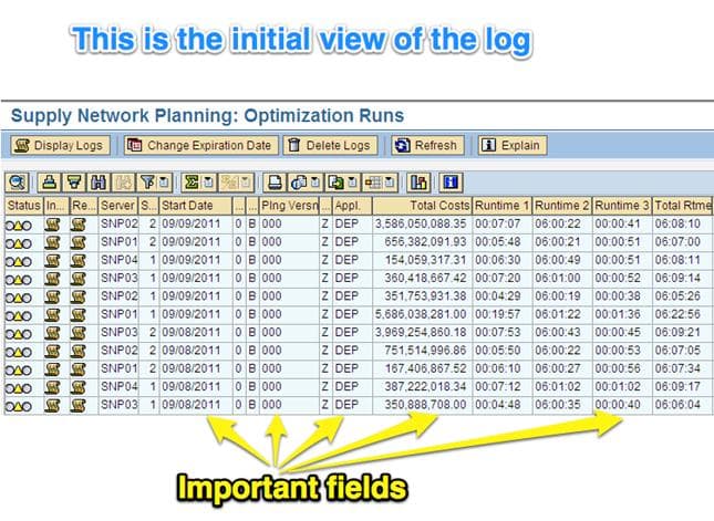
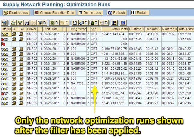
Bullet point all of the fields with definitions

The fields listed above are common fields of interest. This is the Start Date the optimizer was kicked off or started, the Planning Version, which determines if the optimizer was for an active version (which is used by planners). Or applies to a simulation version, the Application, which is whether the optimizer was run for OPT (the network run) or for DEP (for the deployment run), Total Cost, which is the summation of the cost that was calculated by the optimizer, and finally the Total Runtime, which is how long it took the optimizer to run.

The initial log view can be sorted and filtered to find the optimizer log they are looking for easily.

After you have selected the run that you want to drill into, the run can be double-clicked, which will take the user to the screen below.

The log is broken into the segments listed above, which we will now go over.

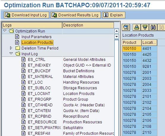
The first area of the log is the Input Parameters. However, there is not much to comment upon in that area. Therefore, the first we will go to is the Location Products.

Location Products View

The Location Products view is simple; you can find what location product combinations were run through the optimizer.

Input Log View

The input log is the next area of the log, and it shows what master data was set up for use in the optimizer. The master data is segmented into many different areas, making it relatively simple to find the master data category of interest.

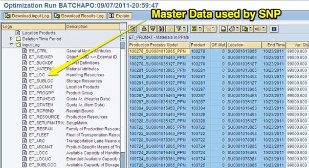
This selection shows the capacity of the PPMs, which is 99,000 cases.

The Results Log View

The Results Log is the next category in the log.

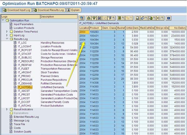
The Results Log shows the output of the optimizer. This is important because it shows what the optimizer decided to do definitively. While the standard planning views such as the Product View and the Planning Book are useful, planners can adjust these views and are not the definitive reference of what the optimizer did. (In this particular subview, which is the Unfulfilled Demands, shows the total unfulfilled demand costs incurred for each location product combination per time bucket. (For instance, at location 2004 for product 114633 for the 14th time bucket, the cost incurred was 4000).

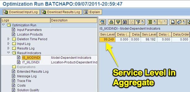
The Results Indicators View

The results indicators display major metrics for the overall run, including multiple measurements for service level and the stock level.

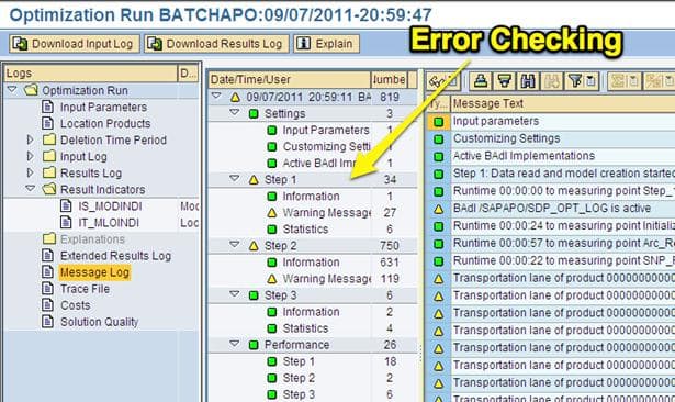
Message Log View

This is the location in the log to look for errors. The errors are organized by the different steps that the optimizer goes through. It also provides the count of each of the different error types. However, it is difficult to determine, in many cases, if the errors are essential. Every optimizer run will have some errors. Many of them are inconsequential. However, problematic optimizer runs have more errors. The errors are essentially pointers to where to go and check the system to make changes.

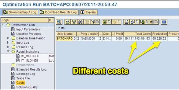
Costs View

Costs are how the optimizer makes decisions. Different categories list the costs in this view, such as production and storage. These are the costs that were incurred by the optimizer during the run. The objective of the optimizer is to minimize the total costs. Unless major changes were made to the model (adding locations, making configuration changes), the costs should be similar from a run to run. An easy indicator of a problematic run has very high total costs compared to previous runs.

Costs are how the optimizer makes decisions. Different categories list the costs in this view, such as production and storage. These are the costs that were incurred by the optimizer during the run. The objective of the optimizer is to minimize the total costs. Unless major changes were made to the model (adding locations, making configuration changes), the costs should be similar from a run to run. An easy indicator of a problematic run has very high total costs compared to previous runs.

Trace File View

The trace file is the master view and file within the log. It contains all of the information that has been discussed up to this point. The trace file also has the advantage of being able to be exported. This is important because APO only keeps two weeks of history. However, by performing successive exports, the logs can be kept as long as is necessary.

The optimizer log is an advantageous transaction containing a large amount of diagnostic information about the optimizer runs. It is not particularly user-friendly.

Analysis of the Issue of the Need for a Full Optimizer Log Trace File

The optimizer log trace file problem surfaced when I began analyzing the optimizer logs in AP1, the production APO environment. I noticed that the log files were not writing a full log trace file. The full log trace file has proven to be a handy tool on my past projects to analyze optimizer results and archiving optimizer results. For instance, I have groups of log trace file extracts from several previous clients. This allows me to compare optimization results across clients at the most detailed level.

Long-term archival of optimization results, as well as a full analysis of results, is one of the largest shortcomings on optimization projects generally and a primary reason most SNP and PP/DS optimization projects operate at a low-level. This is tangentially discussed in this article. I consider this a critical success factor for optimization projects generally.

Responses on the Issue

After discussing the log trace file’s completeness, I learned that a decision was made not to write out the full log file to save processing time with the SNP Optimizer.

Understanding the Differences Between the Standard Log File and the Full Log File

The best way to understand the differences between the current log file and the full log file is to view a matrix like the one I have provided below:

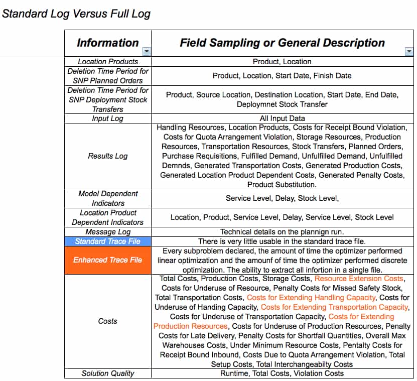
The main difference is listed in the standard trace file versus the enhanced trace file. The enhanced trace file can be saved as an external file and, therefore, archived. One can come back months or years after the fact and review the enhanced trace file. So the difference is both in the quantity of information provided and in its complete form in a single text file. The current optimizer log archival configuration only saves log files back two weeks. After that, the logs are deleted from the system and, therefore, can never be accessed. However, when an enhanced log trace file is extracted, it contains most of the run’s information and can be analyzed at any point in the future. An analyst with a series of extract enhanced log trace files has a powerful and unchanging history of the optimizer runs.

The standard log trace file can be converted through a spreadsheet with macros to provide information in a human-readable form. However, it always requires this translation and still contains less information than the enhanced log trace file.

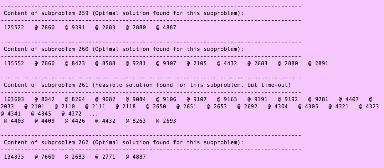
This is an example of the sub-problem enumeration, as shown in the enhanced log trace file.

Issues with the Standard State Log File

The current log file does provide a good level of information, but it also leaves out relevant information. Because the log trace file (a subunit of the overall log file) is so incomplete, it is unusable. It makes it difficult to archive and record how the optimizer has changed over time.

APO Optimizer Security

The topic of SNP optimizer is a subtopic to the subject of APO security more generally. To understand this article, it’s good to have read this article, which describes how authorization is set up in general. Most APO consultants make a pretty lengthy number of excuses for the state of APO security, which range from anything to “this is a training issue” to the “company needs to trust its planners more.” I find it interesting that when functionality is lacking, the debate points seem to gravitate towards other issues. But as I study a variety of best of breed applications, I don’t bring across this horse blinder approach. For those interested in how security should be designed in an application, see my book Bill of Materials in Excel, Planning, ERP, and BMMS Software. The distinctions between average and excellent security will become immediately apparent.

SNP Optimizer Security

The SNP optimizer can be run in two basic ways. One is in the background, where you define the master data selection in a variant as is shown below:

Running the Optimizer in the Background

So, running the optimizer in the standard background mode is a transaction, and in APO – /SAPAPO/SNPOP, I don’t imagine planners would be provided with this transaction.

Running the Optimizer Interactively

However, when running the optimizer through the planning book – called interactively, as soon as the planner selects either the network or deployment optimizer, the planner navigates to the optimizer through the planning book. But once they get to the optimizer, they are no longer in the planning book and instead are taken to new transaction /SAPAPO/SAPLOPT_SNP_GUI.

Therefore, as this is a different transaction, planners can access the planning book but block it from this optimization transaction. If the access is not blocked, there is no additional security below this level – so once they have access, the planner can run every product location in the network. As many companies would like their planners to be able to run “local” optimizations (which is described in this article), the question becomes how to do so in a way that at least provides some accountability so that planners that run the optimizer in an unapproved way can be counseled. This brings us to the next topic, which is the optimizer log. 

Conclusion

This post has been just an introduction to the SNP Optimizer, and SNP Optimizer is an extensive topic, with many settings, diagnostics, and complexities to learn. It is more complicated to understand and implement than either heuristics (comparatively extremely simple) or CTM.

Cost optimization is often set up with costs that undercut the development of global optimums. The costs I included in this article are not unusual. I find it quite common for clients to set one optimization cost category (frequently unmet demand) so high that it is out of conformance with all the other costs in the system and overwhelms the optimizer to meet demand at any cost. However, the concept behind cost optimizers is to minimize costs. This is one of the problems with setting costs entirely divorced from reality.

There can be several reasons why an optimizer will not achieve a global optimum. In addition to using decomposition, some methods can be used to help. However, some enterprise optimizers like SAP SNP do not have these tools. As shown above, only three LP Solution Procedures are available (Simplex, Dual, and Interior Point Method). Without methods to adjust the complexity of the problem and the constraints, solving problems can often require manual divisions or segmentation of the problem into different runs (which always imposes overhead on the solution), removing discrete constraints, and then adding in constraints one at a time.

References

SAP Help

“Real Optimization with SAP APO,” Josef Kallrath, Thomas I. Maindl, Springer Press, 2006

“Optimization Modeling with Spreadsheets,” Kenneth Baker, Wiley, 2011

“Segmentation Problems,” Jon Kleinberg, Christos Papadimitriou, Prabhakar Raghavan, Cornell, 1998

https://en.wikipedia.org/wiki/Simulated_annealing

https://en.wikipedia.org/wiki/CPLEX https://mathworld.wolfram.com/InteriorPointMethod.htmlwhen

https://www.mathworks.com/help/toolbox/optim/ug/br44i40.html#br44j7o “Optimization Modeling with Spreadsheets,”

Kenneth Baker, Wiley, 2011 https://www.egwald.ca/operationsresearch/lpdualsimplex.php

https://www.meiss.com/download/Spreadsheet-Optimization-Solver.pdf

“An Introduction to Spreadsheet Optimization Using the Excel Solver,” Joern Meissern and Thanh-Ha Nguyen, Lancaster University. (date unknown)

https://www.mathworks.com/help/toolbox/optim/ug/br44i40.html#br44i5e

Definition of an Attractor

An attractor is a set of states (points in the phase space), invariant under the dynamics, towards which neighboring states in a given basin of attraction asymptotically approach in the course of dynamic evolution. An attractor is defined as the smallest unit that cannot be decomposed into two or more attractors with distinct basins of attraction. This restriction is necessary since a dynamical system may have multiple attractors, each with its basin of attraction. – https://mathworld.wolfram.com/Attractor.html

https://en.wikipedia.org/wiki/Simulated_annealing