Evidence of The Surprising Consistency of the Supply Chain Planning Process Over Time
Executive Summary
- Background on the history of supply chain planning.
- A fascinating supply chain process diagram from 1946.
- The area of coverage of the diagram.
- A short bio of the diagram’s author.
- What the diagram tells us about system evolution in this area.
The Background on The History of Supply Chain Planning
In a previous article, I explain the history of developing the methods of MRP and DRP. The grandson of Robert E Mitchell was nice enough to send me a diagram that his grandfather developed back in 1946, which is officially titled “Processing the Examination of a Manufacturing Enterprise for Purposes of Planning, Coordination, and Control.” This diagram contains all types of interesting information, and the more I looked at it, the more I found it. Just the diagram’s name gives us information about the framework of the time. The diagram predates the terminology that was eventually standardized in the field. Today it might be called “Integrated Supply Chain Planning Process Flow.” Manufacturing tended to be more emphasized in the past. For instance, materials requirements planning (MRP) was first named manufacturing resource planning until the name was altered a few years after it was first coined. Education at this time could be obtained in industrial engineering/manufacturing, but degrees in what we now know as supply chain management essentially did not exist. If we look back to schools like Penn State and Ohio State, they were some of the very first to start programs in “logistics.” The education in what we now call supply chain management has continued to grow over time and helped spread the understanding that an integrated education in physical delivery systems is an essential field of study.
The Area of Coverage of the Diagram
This is a diagram that shows a complete vision of the connection between the following processes:
- Sales
- Inventory
- Planning
- Material Control
- Purchasing
- Reporting
- Management
- Planning and Direction
- Manufacturing
- Scheduling
- Engineering
This diagram shows or proposes the information that would flow between the various entities. The diagram is too large to show in its entirety and be legible. This diagram has the graphical flows between entitles and detailed explanations of each entity off to the side of the central graphic. The graphic was designed to be printed out on a huge piece of paper (probably rolled up and placed into an architectural cardboard tube for transportation) and displayed on a wall. This would be the kind of document one would expect to find in a project room that people could refer to ground themselves and get on the same page on topics.
The Sales Process
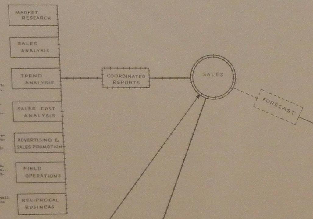
One could begin anywhere on the diagram because it describes a circuit, but as the process tends, start with the forecast, I will start there. Here the diagram shows the relationship between multiple inputs on the left into the sales estimation process. One of the inputs is the available capacity. This today would be called the S&OP process. This S&OP process (sales on the diagram) has two outputs, which we will follow in the next diagram snapshot and explanation. 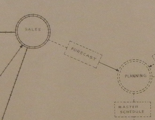
One output is a forecast sent to the “planning” process, which is shown above. The second output is another forecast (which I will not show because the diagram is too long).
The Planning Process
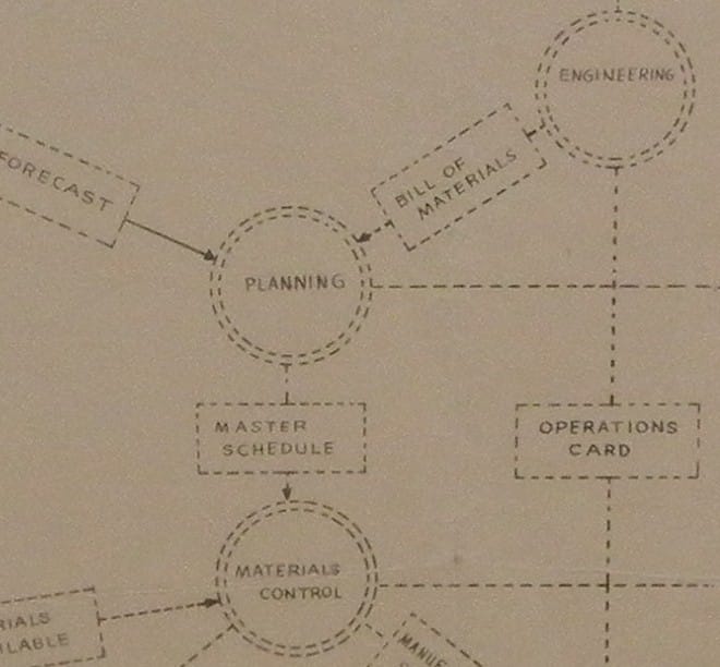 The Planning process also receives the bill of materials from engineering. This is a flow that is greatly underemphasized in supply chain management and is my book’s topic on managing the bill of materials. This portion of the diagram is an excellent way of explaining how this works. The diagram also has associated text, which is quite helpful:
“From this department or from a combination of technical departments comes the analysis of the proposed product in terms of its components and the kind of quantity of material required. For each component to be manufactured, it specifies the method of making it, the machines, tools and gages to be employed, the wait times for each operation and whatever other technical information is necessary to assure a sound basis for production planning, regardless of the quantities or dates. Those data are contained is one of the other four fundamental records provided. ”
The diagram shows these four fundamental records (the BOM, the Master Schedule Prime Materials, Master Operations Card, Tool List) off to the right. Each one of these “records” has a description, which will be too small to read in this rendering: If we go back to the planning process, the portion of the diagram I just showed has two inputs:
- The Forecast (from Sales)
- The Bill of Materials (from Engineering)
It is composed of two primary components (which are decentered to the right on the diagram) are the following:
- Master Components Schedule
- Master Schedule Prime Materials
Interestingly, Robert Mitchell uses the term “planning” more narrowly than I tend to find in projects today. I thought about this and concluded that as this was pre-computerization, the ability to perform planning would have been far less. For instance, throughout the document, the focus is on “orders” and not requisitions, which precede orders in the current time. For example, if I were to use an external planning system, I could rerun the plan multiple times, review the result, and decide when to convert these recommendations to orders. We take this for granted today. However, with the amount of data that had to be processed versus the processing power that existed at the time (that is, human clerks), it makes perfect sense that planning was not something that they could afford to expend much energy on.
The Material Control Process
The diagram has a single output for planning, the Master Schedule, which goes to the Materials Control process. This is a shortened term of the Master Production Schedule or MPS. This is a misleading term because the “master” portion of the word means a subset of planning – and is often confused with the term MRP – which is a method of supply and production planning and is a distinct term from MPS. This is explained in a previous article. (the term has also been confusing and incorrectly used by software vendors adding to the confusion on projects described in this article). Robert Mitchell’s use of the term “Master Schedule Prime Materials,” which is not a term in general usage today, indicates that he is referring to the fact that the MPS he is describing is a subset of the overall product database, which is one of the four ways of restricting the planning run to create an MPS. The MPS is sent to the Materials Control process. This process is made up of two primary components (which are off to the diagram’s right). These are:
- Perpetual Inventory: This term is no longer used and is essentially a pre-software term. I cover this in more detail in this article.
- The Operating Schedule
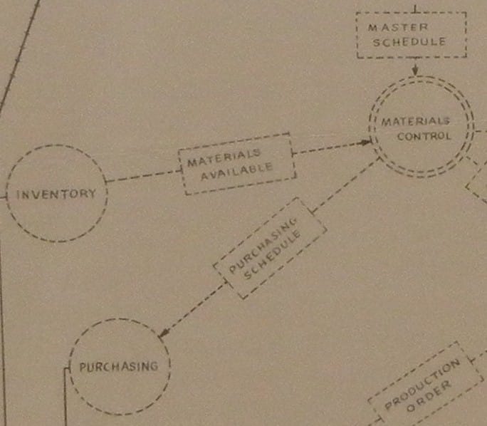
At this point, I noticed something interesting. Today, when a company performs an initial production and supply plan (what is often referred to as an MPS and described in this article on the various threads of supply and production planning). Both the “MPS” and the planned availability, purchase requisitions, and the manufacturing schedule are output as a result of that planning run. However, this combination of factors did not occur until the development of MRP, which did not happen until 1961 (and was not broadly implemented until roughly 1970). This diagram precedes the development of MRP by 15 years and precedes the general implementation of MRP by 24 years. Because of how the software works, we have come to think of the initial supply and production plan and combining the Planning and the Material Control processes (as shown in this diagram). However, this diagram shows that it was not always thought of in these terms. The Materials Control process has three outputs:
- Materials Availability (send to the Inventory Process): On planning projects, we would refer to this as the planned on-hand. This connects and is the input to the available to promise functionality that resides in ERP systems and to a more advanced degree in external planning applications. There is an essential relationship between the quality of the planned on-hand and how far out the available to promise application should commit on orders, which is explained in this article.
- Purchasing (send to the Purchasing Process)
- Manufacturing Scheduling (send to the Scheduling Process)
The Inventory and Purchasing processes’ output goes into what the diagram calls the “Management Process,” which I will cover a bit later. However, the next link we will follow is the Manufacturing Schedule, sent to the Scheduling Process.
The Scheduling Process
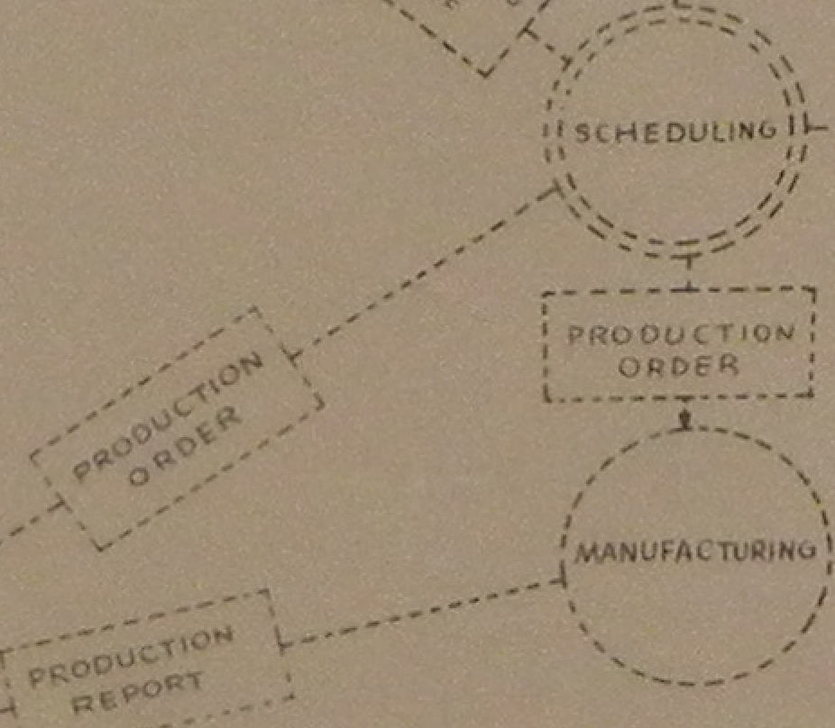
The Scheduling process produces a Production Order, sent to both the Manufacturing process and the Progress process. A Production Report is sent from the Manufacturing process to the Progress process. I recreated this for how I believe this process would appear on a modern project. In this graphic, I have added several items. Some of the items exist but are different once the process flow is placed into a system. The blue font is a new context. The orange font is the completely new item – which is the ERP system confirming the planned production orders back to the planning system. Among the components identified in the poster (and still applicable today) are the Daily Production Report and Material Movement Report. 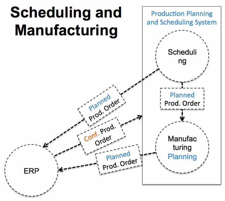
The Progress Process
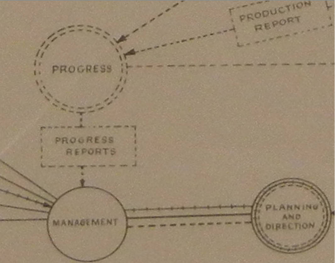
The Production Report is sent to the Progress process, then has a single output to the Management process.
The Management Process
This management process interacts with the Planning and Direct Process and has a Forecast input from the Sales process (which we discussed earlier) and has four outputs which go to the following processes:
- Inventory
- Purchasing
- Sales (which is available capacity)
- Financial and Managerial Reports (which consists of the following:)
- General Accounting
- Cost Accounting
- Payroll and Material Accounting
- Budgets and Control
Historic Supply Chain Planning
I have always been curious how people made planning decisions before the computer and heard many clerks performed calculations. Supply chain management activities were very manually intensive, which limited the sophistication that could be applied. A significant improvement brought by information technology was the simple accounting and calculation that a person had previously performed.
Impressions of the Diagram
When I look at it, I am struck by how modern it seems. If it were not for the paper and the date stamp, I could not tell this was not created last week. Robert Mitchell’s grandson, Pat Michelle, indicated that he had it on his wall at his workplace, and I can certainly see why. I could use the document to explain how planning systems work generally. As I showed previously, to provide any number of modern twists or additions to Mitchell’s diagram.
Interestingly, it looks like it was created with Visio but must have been created with a stencil. 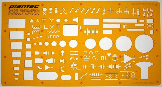 Stencils like this were used long before Visio. Documents like this could have been built on a drafting board with an “arm,” which would allow the draftee to create lines at any angle they wanted.
Conclusion
Overall, it was a fascinating document to analyze and demonstrated how sophisticated the understanding of supply chain planning was even 65 years ago. If we could time travel back to 1946 and walk into Robert Mitchell’s office, we would be able to converse very easily on the topics explained in his diagram. He would not know what an ERP system was, but as long as we kept the discussion at the process level — there would be no problem agreeing on many of the concepts of what is now known as supply chain management. He would have questions for us as time travelers and would undoubtedly be amazed at computers’ development since his time. However, we would have questions for him as well. Much of how companies performed these activities with paper and people and without a calculator has not been very well maintained in books and other publications.
Short Bio of Robert E Mitchell:
I asked Pat Mitchell for a bio of his grandfather, as it is interesting to understand the person’s background that made the diagram.
In 1942, Robert E Mitchell joined Remington Rand as VP of Sales. Remington Rand was a large conglomerate at the time making information processing equipment (typewriters, adding machines) but also handguns and other items. Good history of the company in Wikipedia: https://en.wikipedia.org/wiki/Remington_Rand In the Wikipedia article I found a listing of a book that reviewed the history of the information processing industry including IBM, Remington Rand and others. I found the book in Amazon and found the preface to the 2000 edition very interesting (included in the link below). https://www.amazon.com/Before-Computer-James-W-Cortada/dp/0691050457/ref=sr_1_5?ie=UTF8&qid=1374213673&sr=8-5&keywords=James+W.+Cortada#reader_0691050457 I am not sure if he was the only VP of Sales Remington Rand had at the time or if my grandfather was still in that role when he made that poster in 1946. Prior to Remington Rand, my grandfather worked at Valspar Paint for a number of years and rose to the position of VP of Sales. In 1939 he left Valspar and started a competing Paint company called Paint Engineers that specialized in Industrial paint for bridges and aircraft. He sold a controlling interest in the company to outside investors in order to scale the business but then found himself at odds over corporate direction with the financing team. He left Paint Engineers in 1942 to take on the role of VP of Sales at Remington Rand. – Pat Mitchell
References
https://en.wikipedia.org/wiki/Master_production_schedule
https://en.wikipedia.org/wiki/Perpetual_inventory