How to Understand the Availability Maximization Spare Parts Management Method
Executive Summary
- There is basic parts selection logic of the availability maximizer, which includes the cost of the part.
- Service parts management must be able to deal with zero demand situations.

Introduction
This approach and program were written expressly for a low demand environment at the dealer level. Most independent demand inventory algorithms ( EOQ, POQ, Silver-Meal, Parts-Period Balancing, etc.) rely on the statistics of high demand per replenishment period to determine inventory holding and purchasing amounts. And this brings up the question of the applicability of this environment to low demand per replenishment periods.
The Problem of Applicability of Stable Demand Methods to Spare Parts
For environments with relatively stable demand, these methods work reasonably well. Spare parts demand, in contrast, is generally low in demand per part with significant variability from period to period. As we will find later, low demand and demand variability are related characteristics.
A second limiting factor is that while the spare part demand is low per item, the average spare parts depot will have to carry many times more parts, which must be carried than a manufacturing depot to generate comparable fill levels.
Many Years or Versions of Parts
Spare parts operations must carry not only this model year’s inventories but inventories going back decades.
These three characteristics of the environment of the spare part:
- Low demand
- Highly erratic demand
- Massive parts databases
These all present difficult challenges to a company dedicated to order fulfillment.
Who Owns the Dealership Network?
A second feature of the client’s environment was the client’s lack of ownership of the dealership network.
Many of the dealers sold competing agricultural-construction equipment brands and maintained spare parts for these brands in their stockrooms in addition to the OEM spare parts. Because the dealers would not allow the OEM to manage their inventories with the Availability Max model without experiencing significant benefits, any system used would increase fill and reduce the inventory carrying amounts.
From the environmental challenges described above, it should be clear that the OEMs needed an inventory system much different to address the characteristics specific to its part business.
The Basic Part Selection Logic of the Availability Maximizer
The entire logic within the Availability Maximizer is based on the following inventory goals.
- Limited Resources for Inventory
- Capital Required to Carry Inventory Over Order Intervals
- Physical space in the stockroom at the dealer
- The Company’s Interest in Filling as Many Customer Orders as Possible
These two inventory goals are incorporated into the Availability Max as the following:
- The Cost of the Part (limited resources
- Expected Additional Demand Satisfied (companies interest in filling customer orders)
Why the Cost of the Part?
As was noted in the first section of this paper, due to the low demand per part, the erratic nature of demand, and the vast numbers of parts in a typical spare parts database, a depot would have to carry many times as much inventory as a manufacturing operation of the same general size to generate a comparable order fill.
This is because it would be so expensive.
The typical spare parts operation must accept a certain stock level out on some parts and a 100% stock out on the lowest demand parts in its database. Even after significant inventory intelligence has been used; at some point, the fill level is based upon the aggregate inventory dollars the dealer is willing to commit to order fulfillment. At some point, the customer is no longer willing to subsidize higher fill levels with higher part prices.
Inventory Investment
Therefore inventory dollars investment is a crucial component of order fill—inventory investment composed of the aggregate of all parts in inventory. The inventory system can either buy less expensive parts or fewer more costly parts. Therefore, in the Availability Max algorithm, the cost of the part is the denominator to the objective function, which Availability Max is attempting to maximize for each part.
Why the Additional Expected Demand Satisfied?
Consider yourself in the situation of the parts manager at an OEM dealership. Every week you must decide as to which parts to order. You, presumably, want to order parts that will sell quickly, which would mean your new purchases would take up less space on your shelves, free up monies for further acquisitions, and please more customers.
But, which parts are the best parts to order?
You could purchase whatever you sold the past week, and that would get you part of the way there. Or, you could analyze the previous year’s demand and, with statistical methods, determine the probability of demand on different parts. This analysis would yield the Additional Expected Demand Satisfied, given a certain order amount. The EADS will always be smaller or rare, the same as the amount you chose to order. EADS will never be bigger than the order amount because it is impossible to satisfy the demand for parts you do not have. The calculation of the EADS is simple.
The Current Inventory Position Versus the Yearly Demand
The current inventory position is compared to the yearly demand of the part to determine the probability of additional demand in some multiple of the order size. If the beginning inventory position is small about the lead time demand, then there is a probabilistically larger chance of unfulfilled demand than if the starting inventory position were larger than the lead time demand. ( later in this paper, the specifics of the probability distributions used and their calculations will be expanded upon).
Remember that the second primary objectives for which the model is built are the companies’ interest in filling as many customer orders as possible.
EADS is simply the following formula.
Basic Rule of The Incremental Benefit of Ordering Order Amount (Q)
EADS = % of Q
The Objective Function
The objective function is where the two mathematical expressions of the two inventory goals are put to use. The objective function is the goal that is to be optimized by the Availability Max. In this case, we want the objective function to be maximized.
This will allow the model to select parts that have a high EADS about their cost.
Objective function :
Maximize (Expected Additional Demand Satisfied) / (unit cost)
Determining the numerator, the EADS, to the objective function is where most effort in the Availability Max model is expended. Compared to its probability of being subject to customer demand, a part’s relative cost determines its ranking as either a high or low opportunity part.[1] [2] For two equivalently priced parts, the higher opportunity part is the one with the highest ENDS as a percentage of its order amount. The Availability Max performs the objective function above iteratively.
This means that beginning from a current inventory position, and it calculates the objective function for every part in the parts order amount as many times as necessary. After a single iteration where high opportunity parts are selected for purchase, the purchase amount is then added to the current inventory, and the objective function is calculated again. For the parts purchased in the previous iteration, their opportunity is reduced to reflect those items’ new higher stocking position.
It is important to remember that no part will be identified as a high opportunity for all model calculations. At some point, sufficient inventory is purchased through prior iterations that the part no longer an attractive alternative to adding more stock. To provide perspective, for the average dealer used in this model’s development, it is common for the model to perform 7000 iterations for purchases and returns before arriving at the optimum holding position.
Example 1 shows how the model would choose the parts at different iterations with the demand and cost characteristics in Table 1.
Example. 1
Below are the demand probabilities and costs for part A and part B:
[1] In practice, since there is neither a strong correlation between expensive parts nor cheap parts with demand history, the more expensive parts are at a disadvantage and typically the last to be purchased by the Availability Max. The degree to which it purchases mostly medium to less expensive depends upon the desired overall service level used as an input. The higher the desired service level, the higher the model will purchase on the cost scale.
[2] The model is technically defined as an optimizer. This is because it iteratively compares every part until it finds the optimum combination given the objective function or until it hits a constraint. The constraints are set by the user and include total inventory dollars, new inventory purchases, individual service level, global service level, and iteration cap.
The Brightwork Database and Data Warehouse Scoring Criteria
| Criteria | Criteria Definition |
|---|---|
| 1. Database Type | Does the database fall into the category of a relational, document, column, graph, etc.. |
| 2. Core Market | This is where the database tends to be used with the highest frequency. |
| 3. Memory Optimized or All In-Memory | Determines whether the entire database is run as loaded into memory. |
| 4. Price Score | Prices vary greatly for databases, a major reason being the comparison of open source and commercial databases. |
| 5. Maintenance Overhead Score | One of the least discussed features of a relational database. Maintenance overhead is determined by factors ranging from the SQL used by the database, to the ease or difficulty of configuration to the documentation that supports the database. |
| 6. Licensing / Audit Liability Score | Databases are often purchased without considering the long term licensing and audit liabilities. And even among commercial vendors (there is no auditing for open source), there is a large variance in audit likelihood per vendor, as well as the potential payouts. |
| 7. Usability (i.e Loved/Hated Score) | This score is taken from Stack OverFlow's "most loved and most hated" which is their poll of developers preferences with respect to databases. In the case of HANA, it is not rated by Stack OverFlow, because it is little used, so we inserted our own value based upon feedback from the field on HANA. |
| 8. Functionality Score | This is what the database is capable of doing. This is not a scoring of how easy or difficult it is to bring up functionality within the database. |
| 9. Managed Service / No DBA to Install, Patch or Upgrade | Is the database offered as part of a managed service like that offered by AWS. |
| 10. Autopartitioning / Autoscales | The ability to automatically adjust to scale. |
| 11. Pay Per Section / Per Hour | A function of the availability of the database on cloud service providers that off this capability. |
| 12. Pay Per Storage Used / Not Per Processor | This is a function of how the database is priced. Oracle, for instance, is priced per processor. |
First Iteration .4/5 > .6/8, carry 1 of Part A4
Second Iteration .2/5 < .6/8, carry 1 of Part B
Third Iteration .2/5 >.1/8, carry another of Part A
Final total after three iterations: carry 2 of A and 1 of B
In the first iteration, the probability of a Demand of 1 of Part A divided by Part Cost A. This is compared with Demand of 1 of Part B divided by Part Cost B. However, notice that after the first iteration, the relevant question becomes the probability of a Demand of 2 on Part A vs. a probability of a Demand of 1 for Part B. This is because 1 of Part A has already been purchased. [1] Therefore, the Availability Max model asks, “What is the incremental probability of moving from 1 to 2 demand of Part A vs. the probability of a demand of moving from 0 to 1 demand of Part B.” It is important not to skim over the preceding paragraph as it is the model’s primary operating logic.
The Specifics of the Objective Function for Part Purchases
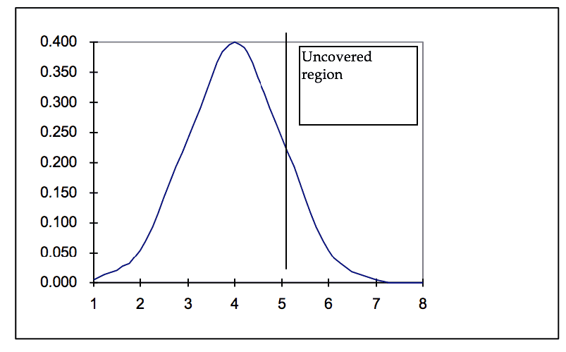
As explained above, the EADS is generated by comparing the current inventory position to the past year’s demand. Given a certain level of demand and a certain inventory level, there is a section under the curve that is left uncovered by the current inventory holding position. Graph 1 displays a situation with a lead time demand of 4 units and an average inventory of 5 units. Demands of 6, 7, 8 units, and above would be stocked-out 1 unit (6-5), two units (7-5), and three units (8-5), respectively. The current inventory will cover any demand up to 5.
Graph 1
Probabilities of Demands Above Inventory Level 5
[1] Two control sets of data were run through the Available Max with the (1- cum service level) opportunity calculation. On one input file, all fields but the cost field were kept constant, and in the other input file, all fields but the demanding field were kept constant. In both cases, the model’s output was consistent. It ordered more higher-demand parts and more low-cost parts. Also, it ordered parts with consistency and the magnitude, which would be expected.
The logic of the model used the formula:
(1-Cumulative probability of (beginning inventory))
This statement would be the mathematical expression of the situation in Graph 1. The output from this equation provides the right side of the distribution (from 5 units and higher), while the following formula would provide the left side of the distribution (from 5 units and lower):
(Cumulative probability of (beginning inventory))
By minimizing the right side of the distribution, (1-Cumulativeprobability of (beginning inventory)), the first version of the model used the correct concept for reducing Expected Demand Not Satisfied, not the Expected Additional Demand Satisfied. For execution purposes, the basic equation of (1-Cumulativeprobabiliy of (n)) was altered to be more robust for the operational version. The following improvement to the basic formula is called the Expected Additional Demand Satisfied purchasing equation.
EADS Purchasing Equation
Q = Incremental increase in inventory (order size)
n = beginning inventory
EXPECTED ADDITIONAL DEMAND SATISFIED = EADS
EADS = -[(Q-1)*PROB.(n+1) + (Q-2)*PROB.(n+2)+…1PROB(N+Q-1)] + Q[1-CUMPROB (n)]
Objective Function = Max ( EADS/(Cost of Part * Q) )[1]
The EADS is a variation of the original formula in that the right side of the equation (in bold) is identical to the original formula. The difference lies in the left side of the equation, which subtracts the current iteration (1,2,3,4, etc..) from the order size (Q) and multiplies this number by the current iteration added to the beginning inventory (n). This equation is performed for iterations from 1 to infinity until the equation’s outcome is sufficiently close to 0. The model is set such that computation of less than .000001 triggers the model to cease calculating this equation.[2]
Rather than attempting to identify the uncovered or unprotected portion of the distribution curve (the right side in Graph 1), the EADS formula determines the size of the incremental increase in the probability of demand (the portion of probability between the lines from a demand of 5 units to a demand of 6 units in Graph 2).
This addition has benefits regarding the model operation, as well as the increased accuracy of probability estimation.
Graph 2
Incremental Probability Added to Fill Rate by Moving from an Inventory of 5 to an Inventory of 6

[1] This (EDS) formula serves as the basis for two other derivations of the Avail Max decision system, one that handles returns and a second, which estimates order fill.
[2] .000001 was selected as it is reasonably close to 0. By setting this parameter, we save the model computation time, which can be better utilized on relevant calculations. This parameter is critical when the model is dealing with parts with higher demand patterns.
Fill Rate Estimation
A second alteration to the Avail Max was performed as to how the model estimates fill rate. The Availability Max estimated the fill rate by just adding the probabilities of demand for the inventory, which were in stock.
For instance, if the lead time demand was four units, and the inventory position of 3 units was chosen as an optimum holding amount. The probabilities of demands of 1,2, and three units were added together to arrive at the estimated fill rate. If, for instance, the probabilities of demands for demands of 1, 2, and three were .20,.25, and .15, respectively, then the model would report a 60% fill rate for that particular part.
The Availability Max estimated fill rate to a useful approximation of order fill by modifying the previous section’s EADS formula. This new fill estimation mimics how one would calculate fill rates on a spreadsheet. Table 2 provides an example of just such a spreadsheet fill rate estimation.
Table 2
Fill Rate Estimation
Examples of fill rates and supporting data.
Inventory Demand Probability Demand Not Filled Probability *Demand Not Filled Probability *Demand
3 6 .05 3 .15 .15
3 5 .1 2 .2 .3
3 4 .15 1 .15 .45
3 3 .35 0 0 1.05
3 2 .25 0 0 .75
3 1 .1 0 0 .3
Totals .5 3
Fill Rate Estimation
| Inventory | Demand | Probability | Demand Not Filled | Probability *Demand Not Filled | Probability *Demand |
|---|---|---|---|---|---|
| 3 | 6 | .05 | 3 | .15 | .15 |
| 3 | 5 | .1 | 2 | .2 | .3 |
| 3 | 4 | .15 | 1 | .15 | .45 |
| 3 | 3 | .35 | 0 | 0 | 1.05 |
| 3 | 2 | .25 | 0 | 0 | .75 |
| 3 | 1 | .1 | 0 | 0 | .3 |
| Totals | .5 | 3 |
% not filled = .5/3 = 0.16667
% filled = 1-.1667 = .8333
The Zero Demand Situation
A third area that improved the Availability Max was in the model’s recognition of situations when there is no demand for a part. With any part, no matter how high or low the prior period’s demand, there is always the possibility that the part will experience zero. With the vast majority of parts in a spare parts database, this probability of zero demand is significant as most parts have demands of less than two units over a two-week lead time.
For example, apart from a Poisson distribution to its demand pattern, which had a lead time demand the previous year of 2 units, it would have a 13.5% chance of not being subject to demand the following year (given use of the naive forecast). This would not amount to a 13.5% fill rate estimation for that part. As the part experienced zero demand, any attempt at fill rate estimation is an illegitimate endeavor, and the Availability Max added the probability of zero demand into its fill calculation.
The fill rate estimation is simply a modification of the EADS formula used to purchase parts. The same algorithm is used with 0 used as the beginning inventory variable (n) and the ending inventory substituted for the order amount (Q). The fill rate is then estimated by dividing the EADS by the mean demand of the past year.
Fill Rate Estimation
Q = ending inventory
n = 0
EXPECTED ADDITIONAL DEMAND SATISFIED = EADS
EADS = -[(Q-1)*PROB.(n+1) + (Q-2)*PROB.(n+2)+…1PROB(N+Q-1)] + Q[1-CUMPROB (n)]
Fill Rate = EADS / Mean Demand[1]
Factoring in Returns
A third change made to the Availability Maximizer was the method by which the model chose to return parts. When first presented, the model used the same logic in the original part purchase equation (EADS). However, this did not run in reverse (returns) very well. It displayed a tendency to minimize the right side (uncovered and unprotected) of the distribution as the order size reduced the current inventory. For the EADS modification (Q), this time, the incremental decrease in inventory is subtracted from the current inventory (n) to generate (z), the substitute factor for (n) to enter into the modified EADS equation.
[1] The Availability Max model contains both a global and individual fill rate cap, which can be entered into the model’s screens before the model is run. The OEM wanted to achieve a global fill rate of 85%. This was introduced before the model ran, and besides, individual caps were set somewhat higher than that level. However, the minimums and package quantities in whose increments forced the model to purchase in larger increments meant that rarely were the individual fill levels close to the global or individual cap. When analyzing the model’s output file, it is essential to remember that the caps do not limit the fill which a single part can attain. They only prevent the model from purchasing additional pieces if the estimated fill rate is above the cap on a particular iteration.
Graph 3
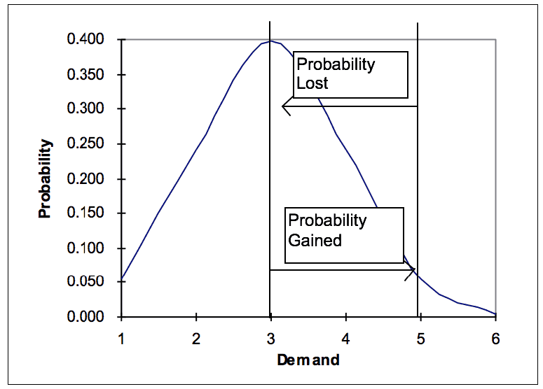
From Graph 3, it is clear that the probability gained of moving from a demand of 3 units to a demand of 5 units ( a purchase quantity of 2) and the probability lost of moving from a demand of 5 units to a demand of 3 units (a return quantity of 2) is identical. Therefore it is only necessary that the formula for a part purchase be modified to generate the probability lost of a return. This is produced by changing the semantics of (Q) in the equation from the order amount to the return amount. This is performed by subtracting the return amount from the current inventory (n) and using the output from this activity (which we call (z)) to enter as a substitute for current inventory (n). This new output could then be called the Expected Demand Lost (EDL) instead of the (EADS).
The EADS Equation (EDL) Modified for Returns
Q = incremental decrease in inventory
n = current inventory
z = n – Q
EXPECTED DEMAND LOST = EDL
EDL = -[(Q-1)*PROB.(z+1)+(Q-2)*PROB(z+2) +…1PROB(z+Q-1)] + Q[1-CUMPROB (z)]
Objective function = Min( EDL/(Part Cost * Q) )
Is This Logic The Correct Logic to Use for Service Parts Inventory Management?
Dr. Hau Lee, Professor of Industrial Engineering at Stanford University, viewed the Availability Max model in operation and recognized it as an application of the greedy heuristic. [1] As it happens, Dr. Lee had jointly published a paper on the greedy heuristic’s use in inventory management. He supports its use for situations with large numbers of parts (a large number of parts, in his opinion, was over a thousand). In experimental results taken from his paper Multi-Item Service Constrained (s, S)[2] Policies for Spare Parts Logistics Systems published in Naval Research Logistics, Lee, Kleindorfer, Pyke, and Cohen used a multi-item algorithm with a Poisson distribution for both high and low demand types.
Two hundred and fifty periods were simulated to reduce any random error. The results were that the greedy heuristic approximation was very accurate, with average errors ranging from .0006 to .031 for low service level requirements, and from .005, to .008 for high service level requirements. The following quote is from the Naval Research Logistics article.
“It is possible to apply a greedy heuristic to both S (order up to level) and s (order point) incrementing with either S or s, for the part and control variable that provides the largest incremental increase in service for the minimum cost.” (570)
The Poisson, the Normal and the Compound Poisson Distribution Assumptions, and the Problem of Specification[3]
To develop the probabilities of different demands for different items for use in EADS and EDL, it becomes necessary to choose a probability distribution that will closely fit the future expected demand. The Normal distribution is used when the demand is sufficient in volume such that the law of large numbers allows for accurate forecasting. (The graphical representations of the Normal distribution can be found in Graph 2, which is up a few pages.) However, for service parts, only the smallest minority of parts fit this description. For the rest, either a Poisson, Gamma, or Compound Poisson s conventionally believed to offer the correct approximation.[4] The Poisson and Gamma are very similar leftward leaning, positively skewed probability distributions. The graphical representations for both are as follows in Graph 3.
Graph 4
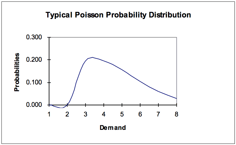
[1]The Poisson and Gamma are positively skewed distributions (positively skewed means that the long tail is in the positive number direction). They are typically used when there is a high degree of randomness in the historical data pattern. Both can be used to predict events like the timing of customers arriving at the bank teller window, trucks arriving at a dock, in addition to the demand pattern for C items. The Poisson distribution has been extensively tested and found to be most effective at approximating future demand when the average lead time demand is below ten units over the test period.[2] [3] The Compound Poisson distribution is used when the demand is both random and extremely “lumpy.”
This distribution is especially applicable when items experience demand in conjunction with one another, for instance, the demand of a left shoe with a right shoe or the demand for complimentary repair parts. The problem with the Compound Poisson is in its calculation, which is complex. In most low-demand situations, either the Poisson or Compound Poisson can be used effectively. The ease of computation was the deciding factor in favor of the Poisson for the Availability Maximizer model.
When the model was first presented, it only used the Poisson distribution. Later the Normal distribution for parts with more than a historical demand of 10 over the replenishment lead time was added. The Normal distribution is calculated in the Availability Maximizer through the use of polynomial exponents displayed below. Polynomial exponents are simply a method for approximating the Normal distribution given a specific normalized value for x.
Polynomial Exponential Approximation for the Normal Distribution
k = ((beginning inventory + Q) – mean demand)/ (standard deviation of demand)
for
(0 <= k <= infinity)
1-.5(1+.196854 * k + .115194 * k2 + .000344 * k3 + .019527 * k4)
Minimums and Package Quantities and Return Thresholds
The model’s logic for choosing parts to buy and hold is known as the “greedy heuristic.” However, while it is single-minded in its search for the best opportunity, it may create uneconomical purchasing scenarios. For this reason, a minimum order quantity on the input file was added. The minimum order quantity was based on an EOQ with an order cost of $5 and a holding cost of .24 per year.[4] Also, to guarantee orders consistent with the client’s system, a package quantity column was entered into the input file.[5] Both minimums and package quantities are used when deciding how much to buy. The first purchase will always be in the minimum order amount, and then successive purchases will be in increments of the package quantity.
However, When returning parts, the minimum field is not used. To ensure that the model did not return parts that may be needed simultaneously, a third column was added to the input file.[6] A nine-month supply of yearly demand generated this column. This was called the return threshold field.[7] [8]
Forecasting
The project’s focus on which the Availability Max model was developed was to test the inventory replenishment logic to select a professional software package that would perform functions similar to the Availability Max. It was decided by the team members that the model would be fed as a naive forecast and that when the software for inventory replenishment was selected, a software package for forecasting would be chosen.
This basic naive approach was further augmented to capture the seasonal nature of the parts of the client. The naive approach was supplemented, as the following paragraphs explain.
For parts with average annual dollar volume x <= $10
If a part has demanded 6 months, then looking forward one and two years ago, use 12 months of demand divided by 2 to generate the bi-monthly demand forecast.
For parts with average annual dollar volume $10< x > $300
If a part has demanded 3 months looking forward to 1 and two years ago, use 6 months of demand divided by 2 to generate a bi-monthly demand forecast.
For parts with average annual dollar volume > $300 parts
If a part has demanded 2 months looking forward to 1 and two years ago, then use 4 months of demand divided by 2 to generate a bi-monthly demand forecast.
When the forecasting software is finally chosen, this methodology would no longer be used. However, the spare parts databases promise challenges that must be dealt with. The vast majority of parts would be classified as C items under traditional inventory theory. According to Silver and Peterson, C parts do not lend themselves to anything but naive forecasts.
However, for a small segment of the database, some parts can be forecasted reasonably well. When we say “reasonably,” we mean better than a 25% forecast error.
Conclusions
In testing, the Availability Max purchased both inexpensive parts and higher demand parts. Spreadsheets that mimicked the logic in the Availability Max were used to test the ordering and return amounts and the corresponding fill rate calculations. These tests to the model’s operating logic indicated the model was selecting parts conformance with its programming. As of the time of this writing, the largest issue is the size of the order minimums. After preliminary runs, the model appeared to be ordering up to the minimum level for most parts. There is evidence that these minimums may be set too high, even though the order cost is only $5 per line.
During the Availability Max development, it was a common occurrence for extra requirements to be projected upon the model. While it may often be intuitively appealing to include all inventory considerations into the model through parameters, there are two drawbacks to this approach.
- Number one, the attempted optimization of more than a few basic parameters can lead to a “middling effect,” whereby the parameters tend to neutralize one another.
- Number two, with each additional parameter, a level of complexity is added to the modeling process. This is undesirable as it requires additional resources from the development team. Second, in developing a day-to-day operational inventory management system, the simplicity of execution is a necessity.
References and Footnotes
[1] Continuous Distributions – specified outcomes cannot be defined, but the range of outcomes can be defined
Discrete Distributions – specified outcomes can be defined, and a range of outcomes can be defined.
[2] Archibald, B., E. A. Silver, and R. Peterson (1974). “Selecting the Probability Distribution of Demand in a Replenishment Lead Time.” Working Paper No. 89, Department of Management Sciences, University of Waterloo.
[3] The Availability Max model does not operate under any lead time parameters. It merely analyzes the demand it is fed as demand over some interval. The manipulation to adjust for lead time is performed on the input file. The project team is currently using a baseline of a two-week total lead time ( review + replenishment ), which means that all parts with demand less than 234 per year fall into the Poisson assumption. This means that less than 100 parts will fall into the Normal calculations in the model for a typical dealer.
[4] Variable order costs ( r ) and holding costs ( A ) are recommended, as it is generally difficult to pinpoint actual costs. For this reason, Silver and Peterson recommend creating exchange curves displaying the effect on order frequency and cycle stock $ with various A/r fractions. At the OEM, while 24% holding cost is un-controversial, the order cost is subject to discussion.
[5] For the model to operate correctly, minimums are always entered as multiple package quantities.
[6] During the project, the OEM voiced a need for the model to deal with non-quantitative issues or issues which were not feasible to put into a mathematical form. These included substitutions, multi-substitutions, and unit of measure issues. The substitution issue dealt with the transfer of demand data from an old part, which had been in some way improved and thus been given a new part number. In some cases, one part may be re-engineered into two parts or two parts reengineered and combined into one part. These are defined as multi-substitutions. As for the unit of measure issues, it was common for the dealer and the OEM to have incompatible data records. For instance, if a hose is regularly sold in 50-foot lengths, the demand data may be corrupted when a sale of one 50 foot length is reported as a sale of “50,” which may be interpreted as a sale of fifty 50 feet lengths. These types of issues were left to “post-processing,” in which the data from the output file would be analyzed on an exception basis
[7] One outcome of these changes is that the model was altered to fit the clients’ day-to-day needs better. A second outcome is that the degree of optimization was effectively reduced as more constraints were placed on inventory purchases and returns. Between individual parts, the fill rates became more staggered. There were many parts with 99% fill rates reported and fewer parts with midrange fill estimations of 83, 86, 92%, etc… With these added constraints, the model chose to leave many parts with no fill rate and others with fill rates well beyond the 85% target.
[8] The model has no time horizon or time orientation. It accepts whatever demand it reads from the input file as the demand over the interval is calculated. If demand over five years were on the input file, the model would calculate an optimal purchase quantity for five years. As we have assumed a two-week total lead time (1 week for review and one week for replenishment), the yearly demand was divided by 26 to arrive at the demand over lead time. The standard deviation used in computation for the probability of demand for the higher demand parts was available to us from the client’s information systems every month. To change the standard deviation to a bi-monthly variance, the monthly variance was divided by the square root of 2.
[1] Lee, Pyke, Kleindorfer, and Cohen. “Multi-Item Service Constrained (s, S) Policies for Spare Parts Logistics Systems.” Naval Research Logistics Vol. 39 pp. 561-577 (1992)
[2] The notation s in (s,S) = reorder point, S = order up to point
[3] The Problem of Specification is defined as the attempt to fit a historical pattern to a probability distribution to use statistical methods on the data. There are a few quantitative techniques, such as the Lillefors test for normalcy. But more frequently, the problem of a specification is resolved by applying probability distributions used for different situations taken from published works.
[4] Another widespread distribution is the Negative Binomial, which is useful for approximating binary events. However, as the Compound Poisson is very similar to it, only the Compound Poisson will be analyzed in this paper.