Setting Up the Planning Area for Aggregated Planning

Executive Summary

• Planning areas must be set up to use SAP APO. To do so, it is necessary to set up the unit of measure and currency.
• To perform aggregation, it is necessary to understand SAP’s explanation of aggregation and aggregation types in SAP APO.

Planning Area Setup

To do begin the first step, it is important to understand all of the options in the planning area. I do this below and emphasize the options related to aggregation.

The planning area is based on the planning object structure. The planning object structure holds the key figures that are used by the planning area. But before we get into the planning area, we will briefly cover the planning object structure, which feeds into the planning area.

“Characteristic Value Combinations (CVCs) are the master data of Demand Planning. They are created from existing InfoCube historical data. These CVCs are stored in the database tables of an APO InfoCube called the Planning Object Structure. This data is independent of the SCM master data transferred by CIF interface. For this reason, in demand planning you can only plan products, sold-to-parties and locations for which you have saved valid CVCs in your planning object structure.” –SAP SCM 220 Training Material

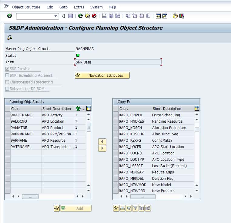
This is a screenshot of the planning object structure configuration screen. Along with the character name, there is a dimension. “A dimension is a component of an InfoCube that is built according to a so-called star schema.

This consists of the following. 

Data Packet, Time and Unit

1. A data packet (cannot be maintained by the user, serves for the consist management of data in the InfoCube),
2. Time (the time characteristics are stored here)
3. Unit (this dimension contains the currencies and units of measure of the key figures of the InfoCube).

“As a result 13, freely configurable dimensions remain at the user’s disposal for the characteristics. Characteristics that are related to one another (such as product, product group, division) should be summarized in one dimension.” Characteristic value combinations define the valid relationships between characteristic values and form the basis for aggregation and disaggregation of key figure values. There are two ways to create characteristic value combinations, individually and automatically. To create an individual CVC, maintain a characteristic value for each characteristic and generate an individual data record in the planning object structure. This is, however, very time-consuming.Alternatively, to create characteristic value combinations automatically, you generate CVCs based on existing data from an SAP BW InfoCube within SAP APO. In this case, the system generates all the combinations that it detects for a particular time period. To maintain the characteristic value combinations up to a date, you periodically schedule a background job that generates the new CVCs based on the most recent sales history. When you update data into a SAP BW InfoCube, such as update the sales order data with a new customer, the background job generates new CVCs for it. This does not erase old CVCs. New ones are simply added.” – SAP SCM 220 Training Material

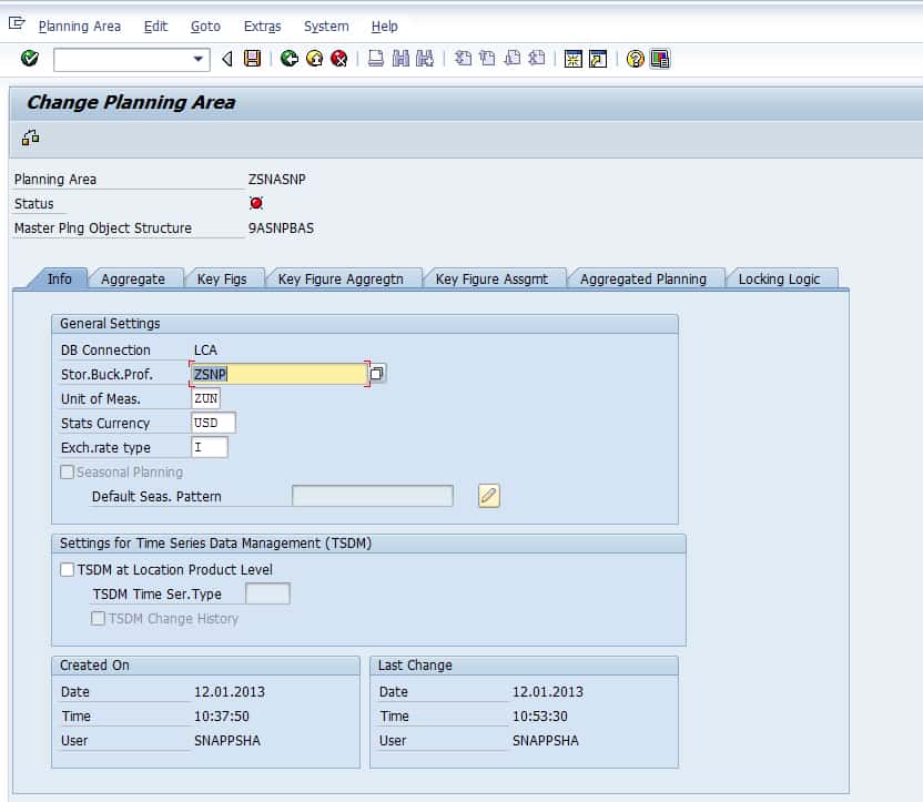
Every planning area must have a planning object structure assigned to it. Notice on this first tab of the planning area called the Info Tab, the planning object structure is at the top and called 9SNPBAS. Notice also that the planning area has a storage bucket profile associated with it as well the storage bucket profile tells the system how to store the planning data. The Storage Bucket Profile is shared between DP and SNP. It defines the periodicities in which you want the data to be saved. This is the lowest level that the date will be divided into intervals in the system. There are two types of timing profiles related to buckets used in APO.

1. Storage Bucket Profile = How the data is stored
2. Planning Buckets Profile = How the data is planned 

Unit of Measure and Currency

Other foundational information like the unit of measure and currency is entered in this tab of the planning area.

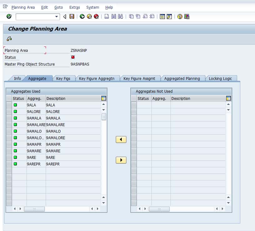
In this tab, the aggregates are set up. This will make more sense when we view the following screenshot. 

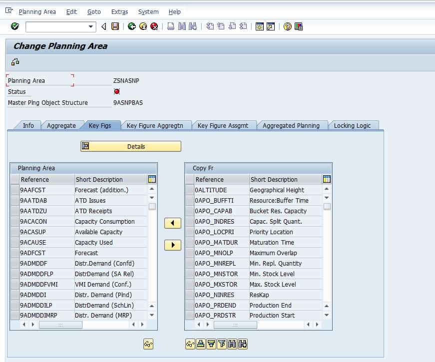
Here are the key figures to the planning area, which are inherited from the planning object structure. Key figures are moved from the right pane to the left pane to be active in the planning area.

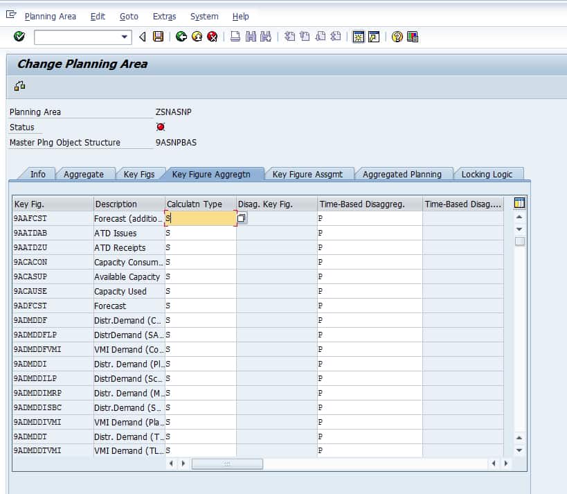
This is the main aggregation screen in the planning area. Two types of disaggregation are configured on this screen. Disaggregation is the act of breaking up an aggregate value and distributing the quantities.

“Aggregation is the automatic function by which key figure values on the lowest level of detail are summed at run time and displayed or planned on a high level; for example, if you display the forecasted demand for a region in the interactive planning table, what you see is the forecasted demand for all of the different sales channels, product families, brands, products, and customers in that region which the system has added together.

Disaggregation is the automatic function by which a key figure value on a high level is broken down to the detailed level; for example, if you forecast demand in a particular region, the system instantly splits up this number among the different sales channels, product families, brands, products, customers, and so on, in this region.”– SAP Help

Rating SAP’s Job of Explaining Aggregation and Disaggregation

Overall, SAP has done a poor job explaining how aggregation and disaggregation work below this high-level definition. This problem extends all aggregation and disaggregation topics across DP and SNP but is pronounced in the following descriptions. Pretty much everyone has an idea of what aggregation and disaggregation are, but the trick to understanding how aggregation and disaggregation work in detail is understanding the calculation type.

Unfortunately, SAP’s definitions have a very “take it or leave it” feel to them, and SAP does a poor job of differentiating between the definitions, making it difficult to understand what each of them does exactly. I have updated these definitions, as well as added a matrix for the calculation types below.

The fields, which control the aggregation, are the following:

“Key Figure: Firstly this is an InfoObject that is assigned to the planning area.[1] Key figures appear in the planning books for DP and SNP. This is the key figure which is to be aggregated and disaggregated.

Calculation Type: Specifies whether and how this key figure is aggregated and disaggregated. This is “how” the aggregation and disaggregation will be performed. This setting is valid for all of the planning books in which the key figure is used. Here are the options:

a.    S – Pro Rata: This is the most straightforward disaggregation. The definition of pro rata is “in proportion” You may have heard a similar term previously, which is “prorated” which means the same thing. However, just understanding the definition is not enough to figure out how pro rata works because pro rata is always proportional to some factor. S- Pro rata disaggregation works in two ways.

If you create key figure values on an aggregate level, the values are distributed on the detail level in equal proportions.

If you change key figure values on the aggregate level, the values on the detail level change so that each value has the same proportion with regard to the aggregate value as before.

b.    P – Based on Another Key Figure: The key figure values are distributed to the detail level in the same proportions as those that can be derived from the values of another key figure. We recommend that you use the calculation type P together with the time-based disaggregation type K.

c.    A – Average of Key Figures: At runtime, the average of the key figure values on the detailed level is shown as the result on aggregate level. When you enter a value on aggregate level, the system disaggregates the value according to pro rata disaggregation.

d.    N – No Disaggregation

e.     I – Pro Rata, Except for the Initial Disaggregation, Which is Based on Another Key Figure: If you create key figure values on aggregate level, the values are distributed on detail level in the same proportions as those that can be derived from the values of another key figure. If there is no value for the basis key figure, the values are disaggregated evenly. If you change data on aggregate level, the values on a detailed level change so that each value has the same proportion with regard to the aggregate value as before. SAP recommends that you use the calculation type I together with the time-based disaggregation type I.

f.     D – Average on the Lowest Level of Detail: As opposed to calculation type A, the system uses the values on the lowest detail level to calculate the average. This can result in different numerical values in comparison to type A. Disaggregation of calculation type D is exactly the same as that of calculation type A.

g.    F – Average at the Lowest Level of Detail that Do Not Equal Zero; Disaggregation According to Pro Rata: The aggregation of this calculation type is basically the same as the aggregation of calculation type D, but in this case does not consider the initial detail values. When you enter a value on aggregate level, the system disaggregates the value according to pro rata disaggregation.

h.    E – Average of all Details that Do Not Equal Zero: The aggregation of this calculation type is basically the same as the aggregation of calculation type A, but in this case does not consider the initial detail values. If you enter a value on aggregate level, the system disaggregates it by copying the value to each detail on detail level.

Disaggregation Key Figure: InfoObject/key figure, which the disaggregation is going towards.

Type of Time Based Disaggregation: This is the second type of disaggregation that can be set in the planning area. This defines how planning data is disaggregated over a period of time. The time buckets in which data is saved are specified by the storage buckets profile. You can use the following time-based disaggregation types:

a.    P – Proportional Distribution: The key figure values are distributed in the storage bucket such that subsequently each value of a storage bucket shows the same percentage proportion for the time-based aggregated value as before.

b.    I – Proportional Distribution: In the case of initial disaggregation, according to another key figure. This disaggregation type is basically the same as type P. However, if a time bucket does not contain a value, the data is distributed based on another key figure. Note: Use the time-based disaggregation type I with the calculation type I.

c.    E – Equal Distribution: Key figure values are distributed equally to each storage bucket. This disaggregation type is only available for key figures that you have defined as not fixed.

d.    N – No Disaggregation in Time: The value in the planning bucket is copied to each storage bucket; for example, a planning value of 100 for the month of June is copied to each of the storage buckets June 1-2, June 5-9, June 12-16, June 19-23, June 26-30. If you show the planned value for June at runtime, the system outputs the average value of all storage buckets. This disaggregation type is only available for key figures that you have defined as not fixed.

e.    K – Based on Another Key Figure: The key figure values are distributed in the storage buckets in the same proportions as those that can be derived from the values of another key figure. Note: Use the time-based disaggregation type K with the calculation type P

f.     L – Read: Value from last period; Write: No allocation: This disaggregation type is intended for time series in Supply Network Planning (SNP). When you aggregate from shorter storage buckets to larger, for instance from weeks to months, the system take the value from the last period and copies it to the larger time bucket. In the reverse case, the value is written to all the smaller time buckets

Time Based Disaggregation Key Figure: This is also an InfoObject which to which the time data is disaggregated.”

This tab shows all the key figures that are part of the master planning object structure. Those are shown to the right. As I indicated earlier, the planning area inherits the key figures from the planning object structure.

[1] InfoObjects divide into characteristics (for example, customers), key figures (for example, revenue), units (for example, currency, amount unit), time characteristics (for example, fiscal year), and technical characteristics (for example, request number). InfoObjects are the smallest information units in BW. They structure the information needed to create data targets.

To the right are the aggregates. If you select the aggregates, it will show more detail to see which key figures are within the aggregates.  

This tab merely points to the planning area to the hierarchy structures that are created in the transaction.   

Types of Aggregation

There are six different types of aggregation available within SAP SNP. One of the six types – the Location Product is a derivative of two other types of aggregation, the Product and the Location, auto-generated from these two hierarchies.

These hierarchy types are listed below:

1. Product
2. Location
3. Location Product
4. Resource
5. PPM/PDS
6. Transportation Zone

All of the hierarchies are created similarly, except for one, which is the location product hierarchy. This hierarchy is created by auto-generating pre-existing location and product hierarchies.

Furthermore, multiple types of hierarchies can be used in the same model.