How to Understand Best Fit Forecast Model Selection

Table of Contents: Select a Link to be Taken to That Section

Executive Summary

We cover best-fit functionality in how it works and the implementation steps in best-fit.
Why the best fit historical accuracy is lower than generally proposed.

Video Introduction: How to Understand Best Fit Forecast Model Selection

Text Introduction (Skip if You Watched the Video)

Best fit forecasting is a procedure within most supply chain forecasting applications. It is a procedure that:

Compares all of the forecasting models within that application for each item being forecasts.
Automatically calculates the error for each model.
Assigns the forecast model to the forecasted item (the product location combination, the product, the product group: whatever is being forecasted)

See our references for this article and related articles at this link.

The Definition of Best Fit

Best fit is a software procedure that is available in most supply chain forecasting applications. It works in the following way generally, although the particulars differ per application.

A software procedure that fits the history using different forecasting models.
The procedure then ranks the various models based on their distance from the actuals or their forecast error.

The forecast model with the lowest overall error is then selected (which is a combination of all the individual errors for every period), and that is the “best fit.”

How is it Run?

Best-fit functionality can be automated within the application (that is run as soon as the application is loaded with data) or require the best fit to be run interactively or as part of a batch job. For example, SAP DP requires the best fit to be initiated in either of these two ways.

How Common is Best Fit?

Almost all statistical forecasting applications have the best fit procedure. However, how much it is deployed is an entirely different question.

Things to Know about Best Fit Forecast Model Selection

Issue #1: Overestimation of Best Fit

Best fit, while sounds nice — is only the best fit of the current models within the application. There are many cases where other models are not within the application that is the best model to use. I have also found cases where the system will not select the best model even though it is in its database.

Combatting Sleazy Consulting Firms

Due to parasitism by consulting firms who try to use our material to cover up for their lack of knowledge our articles to lie to their clients about what they know about best fit, we will not explain this topic in the article, this article will only deal with problems, and will provide no solutions.

Issue #2: Will Best Fit Find the Best Forecast Model?

Best fit will not find the best forecast model in many circumstances.

If the product’s demand characteristics have significantly changed — the best fit determined model is not helpful. For instance, there are cases where the unit of measure changes over time for a product. One product that was sold in one unit of measure changes the unit of measures. In the case there twice as many products are sold — the model selected by the best fit will not catch this — that is, it cannot see the difference between a temporary and permanent change.
The best fit selected forecast model will often underestimate new products. This is because new products tend to build very rapidly.

Issue #3: Applications That Make Best Fit Difficult to Use

Like SAP DP, some applications make the best fit tough to use — and therefore, most of the companies that have SAP DP do not take advantage of its best-fit functionality. I have developed an approach of incorporating the best-fit output of other forecasting applications by using the best-fit model selections in these other applications — and their assignments provided by third-party best-fit results — and building custom models within SAP DP.

This requires patience in the phase of the project where tuning is performed.

An Important Rule Around Best Fit

Best-fit procedures can only say what the best forecast model would have been in the past and cannot be said definitively to be the best model to use in the future.

Common Problems with Best Fit Forecasting Functionality

Common difficulties with the best-fit forecasting functionality are that most companies are mostly related to poorly designed software or poorly designed software from a usability perspective. Best fit forecasting functionality must be controlled to prevent what is known as over-fitting.

The best fit procedure that a forecasting application uses (and different applications have different mathematics that controls the procedure’s outcome) can only tell the user what forecasting models would have worked in the past. This is sometimes the forecasting model that should be used in the future, but it should not be used in many cases. Fitting history is easy; the tricky part is forecasting accurately.

This is emphasized by the well-regarded author, Michael Gilliland of SAS

Michael Gilliland is one of the best sources of practically oriented information on forecasting. He has outlined this practical approach, which Brightwork Research & Analysis supports, in a series of books and articles. In this quotation, he brings up the topic of the historical fit versus the future forecast.

“Historical fit is virtually always better than the accuracy of the forecasts generated. In many situations the historical fit is better than the accuracy of the forecasts. Any one of you who has done statistical forecasting knows this. You might have a MAPE of 5 percent in your historical fit, but a MAPE of 50 percent in your forecasts – that would not be at all unusual. As a practical and career-extending suggestion in communicating with your management, don’t tell them the MAPE of your historical fit – they don’t need to know it! Knowing the MAPE of your historical fit will only lead to unrealistic expectations about the accuracy of your future forecasts.”

Managing Best Fit Comparisons

A best-fit forecast model can be first compared to the naive forecast. Secondly, the best fit can be compared against the current forecasting models to see which accuracy is higher. When a new best-fit forecast is created for a product database, there must be a way of holding it separate from the other forecasts, comparing each of these predictions, and performing analytics to understand the forecast accuracy differences.

In my experience, this often means exporting the different forecasts to Excel (which can now hold millions of records) or a database to perform the comparisons.

Why Can more Complex Methods be Made to Better Fit the Forecast History?

More sophisticated methods can be done to fit the history better, often better than more straightforward methods. This is because they can be tuned to match history better than simple forecast methods. But this does not mean that they necessarily produce a better forecast.

SAP DP

Choosing the right SAP DP model requires patience and multiple runs of the forecasting system, going back and tuning the system, and then rechecking the results. The best way to do this is to use the Univariate view to choose a product or a group of products and make the adjustments.

Groups of products can be selected so that a forecast model and the Forecast Profile adjustments can be checked for all products in the product group. Without best-fit functionality, while grouping products can help diagnostic work, each forecasted product must be checked for the actual assignment. This is a tedious process but necessary for most of the products when using SAP DP.

The best fit can be run from this Univariate view — called running interactively, but as I have already pointed out, the best fit in DP does not choose a particular model that can be efficiently run as part of the batch job. Assignment of Forecast Profiles can be performed in the Univariate view, and these will create a forecast.

Assignment of Forecast Profiles can be performed in the Univariate view, and these will produce a forecast. It often is not feasible to keep the Auto Model Selection 2 assigned as it will usually result in erroneous results (for a reason I will not discuss publicly) – that is, the same pattern will not repeatedly be created.

In most cases, the forecast error can be checked, allowing one to select the best (better) forecasting model type — or Forecast Profile. It is a time-consuming process. It takes too long and is not particularly precise, yet this is the limitation of applying that those who buy SAP DP must learn to live with.

Issues with SAP DP

Many SAP DP customers have not been able to get SAP DP best fit to work correctly and, as a consequence, is eager to get the functionality to work correctly. However, there are some excellent reasons why we have yet to gain exposure to a client that has implemented SAP best fit in a production environment.

Facts About SAP “Best Fit”

SAP has two different best-fit methods: Auto Model Selection 1 and Auto Model Selection 2. What each does is rather involved and takes about 2.5 pages of text and formulas to explain. However, the synopsis is running a series of checks to select the best possible future forecast model given the demand history.

How SAP Best Fit Forecasting is Configured

This essentially sets up different supply chain forecasting methods in competition with one another per demand history trend line. The software goes back in history and uses the previous period to forecast a more recent period for which the actual demand is known. By comparing multiple forecast methods and comparing the error between the forecast and the actual, the software picks a forecast methodology that “best fits” the historical trend.

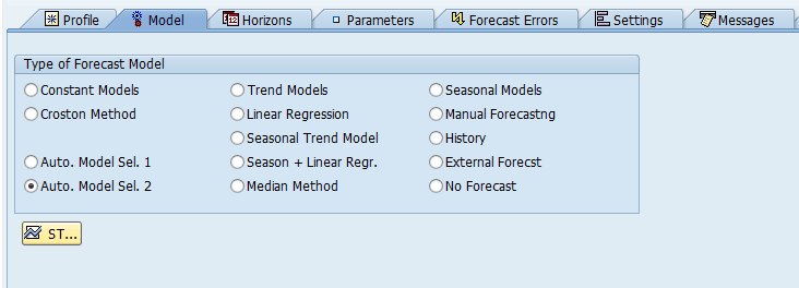
This can do in SAP APO DP by selecting the Auto Model Sel 1 or 2 on the Model tab of the planning book.

The best fit is selected either with Auto. Model Sel. 1 or Auto. Model Sel. 2.

This can be found by going to the options button in the planning book.

Univariate Forecast Profile

The other way to set this is in the Univariate Forecasting Profile. This can be found off the SAP Easy Access Menu:

This takes us right into the Univariate Forecast Profile.

Next, we want to select the “Forecast Strategy” drop-down, which will show the following options. Two of the options are the best fit options, although it is not direct and obvious as to which of these options are the best fit procedures, which is why I have highlighted them below:

It can also be selected from within profile maintenance.

The only decision the planner has to make is the time horizon on which the best fit calculation will be made. This is controlled under the horizons tab in the planning book. Obviously, different time selections can yield different results. However, at account after account, I am finding that this functionality does not work. That returns the constant model, and so clients are not able to use it. Here are two samples.

Best Fit Forecasting Samples

As you can see, the blue line, being the forecast, does not match the yellow line, which is the historical pattern. My client noted the following:

“Auto Selection Model seems to always choose a constant model for the statistical forecast, even when there is a clear seasonal and trend pattern. This does not meet the business’s need to account for seasonality and trend.”

I have told another forecasting vendor about the problems with best-fit supply chain forecasting in SAP DP.

There are two automodel or best fist procedures in SAP DP. This is the Automodel 1 and the Automodel 2. A best-fit procedure is a logical test used to determine which statistical model to apply to a time series.

Understanding Automatic Model Selection Procedure 1

The automatic model selection procedure is used in forecast strategies 50, 51, 52, 53, 54, and 55.

Features

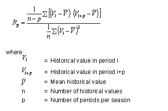
The system checks whether the historical data shows seasonal effects by determining the autocorrelation function (see below) and comparing it with a value Q, which is 0.3 in the standard system.
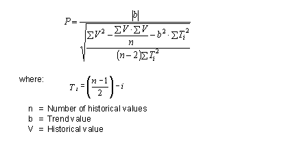
Similarly, the system checks for trend effects by carrying out the trend significance test (formula below).
The formula for Autocorrelation Coefficient

The formula for Trend Significance Test

Activities

Step One

The system first tests intermittent historical data by determining the number of periods that do not contain any historical key figure data. If this is larger than 66% of the total number of periods, the system automatically stops model selection and uses the Croston method.

Step Two

The system conducts initialization for the specified model and the test model (for example, in forecast strategy 54, the selected model is seasonal, and the test model is a trend model).

For initialization to occur, a sufficient number of historical values need to be present in the system. This can be two seasons for the seasonal test and three periods for the trend test.

If not enough, historical values are present in the system for initialization to take place. The model selection procedure is canceled, and a forecast is carried out based on the specified model (in strategy 54, this would be a seasonal model); if the forecasting strategy is one in which no model is specified (for example, strategy 51), a forecast is created using a constant model.

The exception to this rule is strategy 53, which tests for both trend and seasonal models; if sufficient historical values exist to initialize a trend test but not a seasonal test, only a trend test is carried out.

Step Three

In forecast strategies 50, 51, 53, and 54, a seasonal test is carried out:

Any trend influences on the historical time series are removed.
An autocorrelation coefficient is calculated.
The coefficient is tested for significance.

Step Four

In forecast strategies, 50, 52, 53, and 55, a trend test is carried out.

Any seasonal influences on the historical time series are removed.
A check parameter is calculated as in the formula above.
The system determines whether the historical data reveals a significant trend pattern by checking against a value that depends on the number of periods.

Step Five

If neither the seasonal test nor the trend test is positive, the system uses the constant model.
If the seasonal test is positive, the seasonal model is used with the specified parameters.
If the trend test is positive, the trend model is used with 1st order exponential smoothing and the specified parameters.
If both tests are positive, the seasonal trend model is used with the specified parameters.

Overview of Strategies that Use Automatic Model Selection 1

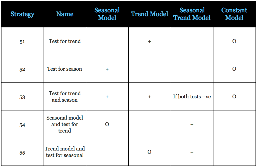
O – default method

+ – a method that is used in the test is positive

Prerequisites

You need at least two seasonal cycles and three periods as historical values to initiate the model. However, if fewer are available, the procedure will run, but models that require more initialization periods, such as seasonal trend, are not used.

Features

The procedure conducts a series of tests to determine which type of forecast model (constant, trend, seasonal, and so on) to use. The system then varies the relevant forecast parameters (alpha, beta, and gamma) in the intervals and the increments you specified in the forecast profile.

If you do not make any entries, the system uses default values, in all cases 0.1. It uses these parameters to execute a forecast. It then chooses the parameters that lead to the lowest error of measure defined in the forecast profile – default is MAD.

Important Note!

For procedure 2, you must bear in mind that when you use the outlier correction, the results are not comparable with the individual processes’ results since another procedure can be selected for the outlier correction than for the final forecast.

Activities

The system then checks for white noise. It means that the system cannot find a model that fits the historical data as there is too much scatter. If it finds the white noise, it automatically uses the constant method.
If both tests are negative, the system proceeds to test for seasonal and trend effects.
The system first eliminates any trend that it finds. To test for seasonal effects, the system determines the autocorrelation coefficient for all possible number of periods (from Number of Periods – Length Variation to Number of Periods + Length Variation). If the most considerable value is larger than 0.3, the test is positive.
The seasonal test is positive. If no seasonal effects have been found, it executes this test for the number of historical periods (as determined in the forecast profile) minus 2. If seasonal effects have been found, the system executes the test for the number of periods in a season plus 1.

Important Note!

Since these two tests’ results determine which models the system checks in the next stage, the Periods per Season value in the forecast profile is significant. For instance, if your historical data has a season of seven periods, and you enter a Periods per Season value of 3, the seasonal test will probably be negative. No seasonal models are then tried; only trend and constant models.

The system then runs forecasts with the models selected (see table below), calculating all the errors’ measures. For models that use forecast parameters (alpha, beta, gamma), these parameters are varied in the ranges and with the step size specified in the forecast profile.

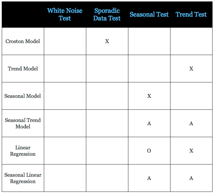
X – The model is used if the test is positive

A – The model is used if all tests are positive

o- – The model is used if this testis negative

The constant model always runs; the one exception to this is when the sporadic data test is positive. Only the Croston model is used (which is a special type of constant model).

The system then chooses the model with the parameters that result in the lowest measure of error as chosen in the Error measure field of the forecast profile.

Recommendation on SAPExpert

On SAPExpert, an article recommends using a macro to perform the best fit functionality. However, this is completely unacceptable. Best fit functionality is “core functionality” for any enterprise forecasting software, and the fact is it should simply work. This type of lying and covering for SAP typical of what is found in SAPExpert and all SAP consulting companies.

Quote From SAPExpert

We found this quote of interest, and it is one of the few quotations, aside from ours, that describes the issues with SAP DP best fit or auto model selection.

Many people have asked me, “Why don’t you use the SAP Advanced Planning & Optimization (SAP APO) functionality for automatic model selection?” This question is easy to answer. SAP APO offers the forecast strategy 50 (automated model selection), but a planner cannot influence the system by choosing a certain strategy since the system decides by itself which strategy to use. In my experience this strategy doesn’t find the best fitting model as it checks only a small set of possibilities and parameters. Wouldn’t it be better if you could select a set of best fitting models in an early project phase and have the system check which model fits the best? SAP APO macros, forecast errors, and process chains can help you solve this problem. First, predefined SAP APO forecast models help you calculate statistical forecasts for all relevant planning objects. Then, the macros allow you to calculate the mean absolute percentage error (MAPE) for all these possible forecasts. Later you compare the different forecasts by checking the MAPE for each model. Finally, you can release the whole calculation as a background calculation by using SAP APO process chains. These process chains can then calculate the forecast models, compare the MAPEs, and find the best fitting model. While there are several ways to approach this situation, this article describes a solution I prefer. The solution I describe here offers several advantages. First, for the user, the whole calculation and the model comparison are done in the background, so you don’t have to worry about finding the best forecast model. Next are the technical benefits. In SAP APO each key figure is stored in SAP liveCache. For every third planning object, key figure, and time bucket, one object in the liveCache must be reserved. These objects are known as Time Series. My method helps to reduce the number of Time Series in the liveCache. Here’s how. Demand planning (DP) often takes place on different aggregation levels. These could be, for example, a material group (bundle of materials with similar characteristics, such as products that are produced on the same capacity line) and the planning material itself (e.g., the different products of a company). One main technical recommendation for SAP APO systems is to keep the planning objects and therefore the amount of Times Series as low as possible. Thus, my recommendation is to do the planning on an aggregated level wherever possible. The process chain functionality I describe here requires at least SAP SCM 4.0 – https://www.scmexpertonline.com/article.cfm?id=4569

Our Analysis

While we applaud SCMExpert for bringing up the issue, in testing using the AutoModel 1 selection (which is one of the best fit models), run in the batch mode, we found SAP DP to provide a superior result to Demand Works Smoothie.

However, on the other hand, it is much more difficult to run SAP best fit. Consequently, most companies do not run either AutoModel 1 or AutoModel 2, except during initial testing, and sometimes to choose parameters for things like seasonality models. However, AutoModel 2 in SAP is completely unusable and has been since we began working in DP years ago. Secondly, AutoModel 1 does not give the same results when run interactively as it does in batch, which is a known problem.

Macros for Best Fit as a Recommendation?

On the topic of SCMExpert’s recommendations to use macros to replace the best fit functionality, we have a serious philosophical problem with this recommendation. Macros should not be used for what is really core functionality in an application. They are designed to provide calculated values in the Planning Book and to extend the basic functionality in DP, not replace it. If companies dislike DP’s best fit functionality and want something more comfortable to use, instead, we would recommend using it in an inexpensive prototype environment to perform this function.

Univariate Forecast Profile

The other way to set this is in the Univariate Forecasting Profile.

Next, we want to select the “Forecast Strategy” dropdown, which will show the following options. Two of the options are the best fit options, although it is not direct and obvious as to which of these options are the best fit procedures, which is why I have highlighted them below:

It can also be selected from within profile maintenance.

Issues For Which DP Best Fit is Blamed but Which are Not Its Fault

In addition to the real issues described above, DP Best Fit is often blamed for things that it has nothing to do with. The most common is that Auto Model 2 will return a constant model for items that have an erratic demand history when running in the batch. This result is typical of all forecasting systems with the best fit functionality and, in fact, is logical for any system to do in this circumstance. This result offers a clue to companies regarding what to do with these products. This is a cue that most individuals and businesses have not picked up on.

Go to top

Conclusion

What to do with SAP DP Best Fit can depend on the client. However, some standard things can be done to improve Best Fit. Best fit in companies that use DP is always a problem, and it has been since DP was first introduced.

(As a note, this article was updated in February 2021, and nothing has changed since this statement was first made. DP is currently at the end of life with new development going into IBP, so it will likely not change in the future.)

A company must triangulate Best Fit’s output with a prototype environment’s results to know the results are correct. We also work with planners to provide them with more transparency into the best fit results and pick the SKU-Locations that should use the best fit selected forecasting method and those that should not.

Our Recommendation

This and several other experiences have led me to not use the standard best-fit

Comparative Design Rating

So I would rate both the above solutions are roughly equal concerning the ease by which the best fit can be initiated.

Regarding the setup for SPP, my intuition is that this configuration is over-engineered and that clients would prefer something more simple in this area. Knowing what I know about the more restricted budgets in service parts accounts, I would have made SPP more simple and with fewer areas to customize vs. DP and SNP, not more complicated.

Issues With Best Fit

One of the major factors that is left out of best fit analysis is being able to measure forecast error for large numbers of line items in an automated fashion.

Why Do the Standard Forecast Error Calculations Make Forecast Improvement So Complicated and Difficult?

It is important to understand forecasting error, but the problem is that the standard forecast error calculation methods do not provide this good understanding. In part, they don't let tell companies that forecast how to make improvements. If the standard forecast measurement calculations did, it would be far more straightforward and companies would have a far easier time performing forecast error measurement calculation.

What the Forecast Error Calculation and System Should Be Able to Do

One would be able to for example:

Measure forecast error
Compare forecast error (For all the forecasts at the company)
To sort the product location combinations based on which product locations lost or gained forecast accuracy from other forecasts.
To be able to measure any forecast against the baseline statistical forecast.
To weigh the forecast error (so progress for the overall product database can be tracked)

Getting to a Better Forecast Error Measurement Capability

A primary reason these things can not be accomplished with the standard forecast error measurements is that they are unnecessarily complicated, and forecasting applications that companies buy are focused on generating forecasts, not on measuring forecast error outside of one product location combination at a time. After observing ineffective and non-comparative forecast error measurements at so many companies, we developed, in part, a purpose-built forecast error application called the Brightwork Explorer to meet these requirements.

Few companies will ever use our Brightwork Explorer or have us use it for them. However, the lessons from the approach followed in requirements development for forecast error measurement are important for anyone who wants to improve forecast accuracy.

Go to top

Conclusion

The best fit is not universally applicable to all products in a forecasting database. Some applications make using the best fit (when applicable) very smooth. SAP DP uses best fit difficult, which is especially problematic because SAP DP Forecast Profiles takes a while to tune. This both stretches the business’s patience and causes the business — which is most often not funded to support such an application like DP, which has so much maintenance involved.

At one time, it was thought that the best fit could always be used to perform the right selection. This is something promoted not only by SAP but many software vendors. And it is entirely untrue. Several clients, I have worked with enabled and then disabled best-fit forecasting in SAP DP. I cover this topic in this article.

Notice

It has come to our attention that Guidehouse Consulting has been using our best fit material to try to figure out the best fit for the US Navy. Guidehouse Consulting has reached out to us to provide free consulting support. If you have a consulting firm that is struggling with best fit or auto model selection, you most likely should not have them as a consulting firm as most consulting firms have no idea how to get this functionality to work. Companies like this one are why when have decided to remove solutions from our articles.