
How to Best Understand the Limitations of the Economic Order Quantity Formula
Executive Summary
- The Economic Order Quantity (EOQ) usually is not analyzed before using it.
- We cover the limitations of EOQ.
Video Introduction: Standard EOQ Formula
Text Introduction (Skip if You Watched the Video)
The EOQ formula is used to determine order batching. Order batching is a method of setting the order size such that it is considerate of various costs and considerations. Order size is something that we naturally do when we shop at a grocery store, although it is done more by feel than by calculation. EOQ is a well-known formula but is far less commonly used than generally through. You will learn about the assumptions of the EOQ formula and when EOQ applicable.
Our References for This Article
If you want to see our references for this article and other Brightwork related articles, see this link.
What is the Standard EOQ Formula?
Economic order quantity (EOQ) is one of the oldest formulas in inventory management. Ford W. Harris first developed it in 1913. Since its introduction, EOQ has been one of the most important and most durable formulas in inventory management.
- Since its introduction, EOQ has been one of the most important and most durable formulas in inventory management.
- It contains some essential assumptions of the EOQ model that are often undiscussed but important to correctly use the formula.
George Plossl on the Assumptions of Economic Order Quantity
Economic order quantity is discussed as a vital consumption-based parameter to set. George Plossl points out in the book Production and Inventory Control; some critical assumptions of economic order quantity make the use of EOQ valid.
This quotation related to economic order quantity assumptions is listed below:
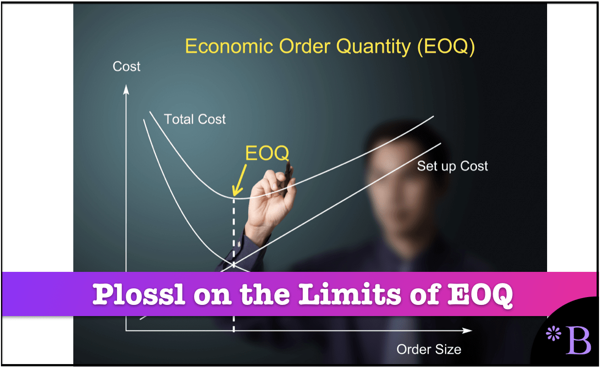
The right quantity to order is that which best balances the costs related to the number of orders placed against the costs related to the size of the orders placed. When these costs have been balanced properly, the total cost is minimized. The resulting ordering quantity is called the economic lot-size, or economic ordering quantity (EOQ). The EOQ concept applies under the following conditions: The item is replenished in lots or batches, either by purchasing or manufacturing, and is not produced continuously. Sales or usage rates are uniform and are low compared to the rate at which he item is normally produced, so that a significant amount of inventory results. The EOQ concept does not apply to all items produced for inventory.
In a refinery or on an assembly line, for example, production is continuous and there are no lot-sizes as such. The bulk of the jobs in a make-to-order plant are made lot-sizes ordered by the customer. Limited tool life, short shelf life, economical price of raw material and other constraints override the application of EOQ techniques. Nevertheless, the concept has broad application in industry, since most production is not continuous and individual lots of material are being taken from one inventory, processed and then delivered to another inventory. – George Plossl
Assumptions of the EOQ Model
- EOQ assumptions are critical in determining the applicability of EOQ to a scenario.
- The EOQ model assumes that costs can be traded off. With the standard EOQ formula, the assumptions EOQ model is that holding costs and ordering costs are the costs to be used.
How to Use the EOQ Formula for Pull Forward or Stock Building
Economic order quantity is one of the oldest formulas in inventory management. However, it is not an adjustable formula; unlike the dynamic safety stock calculation, it cannot account for variability.
Therefore, it must be periodically recomputed for the entire product location database.
When is the EOQ Formula Applicable?
EOQ is used in conjunction with reorder point (see this link for the Reorder Point Calculator, and it applies under similar circumstances:
The item is replenished in lots or batches, either by purchasing or manufacturing and is not produced continuously.
Sales or usage rates are uniform and are low compared to the rate at which the item is produced, so a significant amount of inventory results. – Production and Inventory Control: Principles and Techniques
However, economic order quantity can be used in circumstances where sales vary over the year by changing the EOQ value. This is another reason why it is good to perform an external calculation of supply parameter values that can be adjusted and then uploaded to a system.
How the EOQ Formula Can be Adjusted before High Periods to Build Inventory
Companies often receive a disproportionate amount of demand in one reoccurring period. The EOQ value can be adjusted and then uploaded to the supply planning system in advance of this increased demand to build inventory to the right level more economically. There are two differences regarding doing this versus using the standard EOQ calculation.
- The timing must be right – that is, the broader economic order quantity formula must be calculated sufficiently ahead of the demand increase.
- Add the percent increase to the calculator.
How the Economic Order Quantity Formula Calculation Form Works
This form requires input to provide output. However, it also has default values. You can change any input value and the rest of the formula — the output will change immediately. You can continue making changes, and the form will always update without having to press any button or refresh.
This calculator assumes that the location receives the entire order at one time. However, this assumption does not always hold. For the non-instantaneous receipt, the EOQ calculator read the article EOQ Calculator Noninstantaneous Receipt.
What Economic Order Quantity Can’t Consider
EOQ is designed for stable demand situations. What will follow is a list of anything but steady state; however, EOQ is not the only approach to inventory planning that has difficulty managing these situations.
Item #1: Seasonal Production
Many products have a seasonal sales pattern. It is not unusual to see much of the anticipated requirements produced well before the season to keep production reasonably level throughout the year. During this inventory building, the inventory that is being added is anticipation inventory, not lot size inventory, and the regular EOQ model does not apply.
Instead of balancing ordering costs against inventory, the company is now trying to store staff hours. For this reason, many seasonal items are produced in one lot size per year.
Item #2: Assembly Lot Sizes
Another typical situation encountered in real life is determining lot sizes for assemblies and their components, and once again, the extreme conditions present the clearest examples. An assembly composed of unique elements not used on other meetings should have its lot size calculated, considering all setup costs for the assembly’s components. Most of the components should be manufactured in the same lot sizes as the assembly.
Item #3: Die Life
Costs associated with limitations, such as the life of a die set used in a blanking press, are seldom included in the EOQ formula. The calculated EOQ for an item might indicate that 20,000 units were the most economical lot size, whereas the normal die life might be 30,000 units. Because of the high cost of regrinding, refitting, and setting up a die, it is almost always practical to tie the economic lot sizes into the die life.
In this case, the calculated lot size would probably be increased by 50,000 units.
Item #4: Space Costs
There is no specific allowance in the simple EOQ formula because the space cost for different items can indeed be different. Shipping cartons usually have a low unit value, a desirable discount schedule, and take up vast amounts of storage space.
On the other hand, electronic components have a very high unit cost and take up very little storage space. Especially with bulky items, an estimate of total space requirements resulting from EOQ calculations is essential.
Item #5: Actual Run vs. Order Quantities
The author’s experience that ordering quantities indicate on records and the ordering quantities used in the factory can frequently be quite different. Comparing new lot sizes with the present order quantities to determine the effects and economies of change should be based on the actual lot amount being processed in the plant, not the amount requested by the production control department.
Item #6: Hold Points
“Many items are dealt with by a sequence of operations. The ordering cost must then include the sum of the setup costs for all operations. If set up on one of the early operations is a highly substantial proportion of total setup costs, it may be economical to establish an inventory called a hold point beyond this high setup operation.” – Production and Inventory Control: Principles and Techniques
This same emphasis is covered with a procedure rather than EOQ in this link on pulling production forward.
How to Best Use the EOQ Calculator with Non-Instantaneous Receipt
There are many EOQ formulas or EOQ models — each for a different environment and different problem. However, this is the EOQ model used in most supply planning systems — although it does not necessarily make it the right EOQ model to use for your business or different segments of the product location database.
George Plossl brings up this point well in the following quotation:
“Frequently, for example, the entire lot size is not received into stock at once. The manufacturing rate may be such that it takes several days or even weeks for the complete lot to be made and delivered into stock. While production is going on, partial deliveries to stock are made, but withdrawals are also made during the period. Consequently, the average lot size inventory will not equal one half of the lot size, as it does where all the lot is received at once. This situation, given the rather formidable name of non-instantaneous receipt, can be handled by using a modification to the basic EOQ formula.” – Production and Inventory Control: Principles and Techniques
The EOQ model he is referring to replaced the denominator of the inventory carry cost with the inventory carrying cost (as a decimal fraction per dollar of average inventory * (1-the usage rate, in the same units as the production rate divided by the production rate), which is emulated in the form below.
- These modified formulas are not available within any supply planning system I am aware of.
- This is why we have been promoting the concept of calculating EOQ outside of the systems through supply planning parameter optimization and then uploading this to the system as a stored rather than calculated value. This is how to arrive at an optimal order quantity calculator.
How the EOQ Model Calculation Form, Optimal Order Quantity Calculator Works
This form requires input to provide output. However, it also has default values. You can change any input value and the rest of the formula — the output will change immediately. You can continue making changes, and the form will always update without having to press any button or refresh.
Specific Problems with Lot Sizes
Specific problems with lot sizes come down to first — determining the specific factors to use, which is always a question described by the previous quotation.
Secondly, the factors that are used are not as stable as the quantities change. George Plossl explains this in the following quotation.
“The use of formulas to calculate “economic” order quantities poses several significant problems. The assumption made in the formula derivations that inventory carrying costs and ordering costs vary uniformly with lot size are generally not valid. These costs cannot be assigned a specific, constant value over a range of lot sizes; this value will vary with the total inventory. Either too large an increase in inventory or too many orders being generated can result from application of the formula.”
Therefore, while ordering costs (and if the item is produced, it is ordering costs setup or changeover costs) are considered the same regardless of the quantities involved, when does this not hold in reality?
To further this point, the estimation of precise changeover costs is quite difficult because it depends on what product is being transitioned to. For instance, observe the following changeover matrix.
Forecast Error from Component Interchange-ability
| Material Type | Material | January Forecast | January Demand | Individual Forecast Error | Combined Forecast Error |
|---|---|---|---|---|---|
| Average Error | 11.25% | 2.8% | |||
| Finished Good | Table Type 2 | 150 | 165 | 10% | |
| Finished Good | Table Type 1 | 200 | 175 | 12.5% | 2.8% |
Notice that the changeover value depends upon what value is being changed over from and to. However, lot sizing must be set up without knowing what the from and to products are (unless the lot size is computed each time manually). Although it sounds appealing, using an average will not help, as in most situations, the average value is too far off the actual value.
The following quotation goes a step further and critiques the benefits of dynamic order quantities.
Dynamic Order Quantities
A dynamic order quantity allows the system to change the quantities ordered rather than ordering the same amount for each order. Dynamic order quantities are most definitely the status quo in how MRP is run in companies.
“Dynamic order quantities are a mixed blessing in an MRP environment. While they reflect the most up to date version of the materials plan, they change frequently the item’s component requirements and thus also their planned coverage. A re-computation of a parent planned order quantity will often cause MRP to reschedule component item released orders, in addition to revising planned order quantities and schedules in future periods.
While some nervousness inevitably arises in normal operations, it can be greatly amplified by lot sizing techniques recomputing lot sizes automatically. This can and should be avoided. Many users of MRP systems freeze quantities of planned orders within the span of the cumulative product lead time, so that these orders cannot change gross requirements on lower levels that may be covered by replenishment orders already released.”
How Should EOQ and Other Supply Planning Parameters be Calculated?
One would be able to, for example:
Item #1: Simulation
Set the supply planning parameters in a way that one can simulate the impact on the overall supply plan. When using supply planning systems, inventory parameters are typically managed on a "one by one" basis. This leads to individual planners entering values without considering how inventory parameters are set across the supply network.
Item #2: Interactivity of Changes
This is the ability to see the relationship between changes to service levels and the simulated output.
Item #3: Seeing Financial Implications
This is the ability to see the impact on the dollarized inventory for different aggregate settings.
Item #4: Mass Change for Efficient Maintenance
This allow the parameters to be changed en mass or as a mass change function. Both supply planning systems are designed to receive parameters; they are not designed to develop the parameters.
 Getting to a Better Parameter Setting Capability
We developed an approach where EOQ and reorder points are calculated externally, which allows for a higher degree of control. And for the average inventory to be coestimated in a way that provides an observable total system inventory, holding cost, service level, and a picture of what is happening to the overall system. Calculating individual parameters like EOQ without an appreciation for the systemwide does not make any sense. Also, in many, perhaps even most cases, there is no reason to use EOQ for the purposes given above. Instead, an alternative custom order batching method can be created to replace EOQ. There is nothing magical about EOQ. It is not a "best practice." It will not provide you with "digital transformation." It is not "Six Sigma." You will not get a "black belt" for using it.
After observing ineffective and non-comparative supply planning parameter setting at so many companies, we developed, in part, a purpose-built supply planning parameter calculation application called the Brightwork Explorer to meet these requirements.
Few companies will ever use our Brightwork Explorer or have us use it for them. However, the lessons from the approach followed in requirements development for supply planning parameter maintenance are important for anyone who wants to improve order batching and supply parameters.
Conclusion
These are interesting observations that are not brought up with much frequency. George Plossl, one of the deepest thinkers on MRP and inventory management, apparently emphasized reducing nervousness in the plan. I have found it very difficult to get my clients to take this position — whenever possible, the preference seems to be updated as frequently as possible.
The history of the development of economic order quantity turns out to be interesting. It’s a story of how a high school educated engineer made the most enduring inventory management contribution. But most companies that use EOQ are unaware of the EOQ assumptions of economic order quantity. This leads to things like applying order costs, which are too low and reducing EOQ’s overall usefulness.
There are many economic order quantity formulas to choose from, each with different EOQ assumptions. Therefore, if one does not fit the requirements’ EOQ assumptions, another EOQ formula can be used.
The vast majority of applications only provide a small number of economic order quantity formulas to choose from, but any EOQ formula can be calculated outside the system and imported.
- EOQ can only see the fundamental trade-off between inventory cost and order cost — therefore, it must be adjusted to account for different scenarios.
- A common misperception is that more sophisticated methods handle these issues listed above. In a few cases (such as seasonality & space costs), this can be true, but it is almost always not the case in actual live systems. It can be easier and more straightforward to account for these factors through parameter calculation, as is explained by our application, the Brightwork Explorer.