
Test Results: Quarterly Versus Monthly Forecasting Buckets
Executive Summary
- This test was performed to test a common proposal by customers that smaller forecasting buckets lead to higher forecast accuracy.
- This test was performed with time-based forecasting disaggregation to enable an apple to apple comparison.
Introduction
It is common for companies to consider moving towards a weekly statistical forecasting bucket for supply chain management. I recently came upon a company that had already moved towards weekly forecasting planning buckets. I brought up the topic of monthly forecasting planning buckets, and they asked me why I suggested that. In my previous Test Results from Monthly Versus Weekly Forecasting Buckets, I covered the testing of using a monthly forecasting bucket and disaggregating to a weekly bucket to compare against a forecast created with a weekly bucket.
See our references for this article and related articles at this link.
The results of the study were that for the data set that I tested, which was from an actual client, it was better for the forecast generated in a weekly planning bucket (using sales history also in a monthly planning bucket).
After this, I became curious as to whether the forecast accuracy could be further improved by moving to an even larger forecast planning bucket. In one meeting, my client asked me that if I thought monthly would be good, why not quarterly. So I thought why not see if quarterly planning bucket – disaggregated to a weekly forecast would be a further improvement.
Getting the Forecasting Timing Terminology Correct
To begin, as with the previous article, I wanted to distinguish the following forecast timings before we get into this topic in depth.
These are the most important timings in demand planning:
- The Forecast Generation Frequency: This is how frequently the statistical forecast is generated.
- Forecast Horizon: This is how far into the future, the forecast is generated.
- Forecast Planning Bucket: This is the increment of time for which estimates are produced – most commonly in daily, weekly, or monthly buckets. In most cases, the planning bucket corresponds to the forecast generation frequency, so that you would generate weekly forecasts each week, monthly forecasts each month, etc. However, this is not essential. The planning bucket could be longer or shorter than the forecast generation frequency.
For this article, we will only be discussing the last timing, the planning bucket, and not covering the first two timings except where we need to explain when these other timings are incorrectly commingled with the planning bucket timing. In my experience, planning timings are some of the most confusing aspects of the subject. For instance, what does the term” weekly forecasting” even mean? I could be referring to the Forecast Generation Frequency, or to the “Forecast Planning Bucket.”
One can predict by looking at these two model selections compared that the second selection would have a lower forecast error. However, in cases where companies perform weekly ordering, that is not sufficient. One must prove that when the monthly forecast is disaggregated to a weekly forecast that the forecast error will be lower than when a straight weekly forecast is generated.
That was what was tested.
Testing the Hypothesis
This hypothesis was tested with client data as part of a forecast improvement project. The client did not ask me to test this. However, after the results of the first test that showed better forecast accuracy forecasting at the month, I was curious as to how the quarterly forecasting bucket would perform. So I tested this on my own time. The idea from the client when offered the test was that conducting such a test was just not a good use of time. In their view, the test was just too weird to be worthwhile.
Before we get into the results, let us discuss the method used for performing time-based disaggregation, or in more basic terms, how I disaggregated from the quarterly generated forecast value to a weekly value.
Time-Based Forecast Disaggregation
Time-based aggregation needn’t be that complicated. Frequently using something similar to the actual breakdown of the days in a month will do. This might be something like the following: 21%, 21%, 21%, 21%, 18% (for the last week of a five-week month), and this means applying this disaggregation per week, but normalized for a quarter. There may be 13 weeks in a quarter, so 21% can be normalized for the quarter to result in 7%.
Let us review the forecast models that were applied to the monthly forecasting bucket.
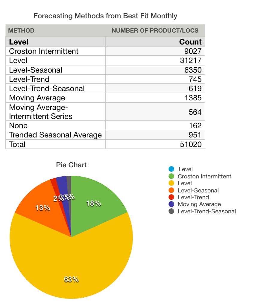
Now let us see the models assigned to the quarterly forecast bucket.
Notice the models were again improved with the percentage being applied to Crostons’ declining again.

- Although a lot that happens here is positive, something also happened that is not positive. Notice that the seasonal models completely fell out of the selection.
- I commented to Bruce Weiland in the previous article that:
“A seasonal index can be applied at a week or even a day, but I believe that seasonal models are designed for a larger time bucket than a week and probably a month. In the next test I will see what happens when I aggregate to a quarterly time bucket.”
The fact that I guessed right is indicative that yes, you undermine the ability to use seasonal forecast models once you move to a quarterly time/planning bucket.
Reducing the Seasonal Models due to the Time Bucket
Deprived of the use of seasonal models due to the time bucket selected, I could have further improved forecast accuracy with the application of seasonal models. However, I am performing these tests without manual intervention. This is a test of how the best fit procedure responds when placed under different temporal aggregations. A future test could be done, which keeps that hard assignment of all seasonal models while allowing product location combinations without the assignment to seasonal models when forecasted with a monthly planning bucket to be freely reassigned to new forecast models with the best fit procedure.
A future test could be performed, which keeps that hard assignment of all seasonal models while allowing product location combinations without the assignment to seasonal models when forecasted with a monthly planning bucket to be freely reassigned to new forecast models with the best fit procedure.
The Test Results
What I found is that the forecast error for a disaggregated quarter was lower than when compared to the forecast generated for a month and disaggregated to a week, or simply a forecast produced at a weekly forecast bucket.
- It was 2.5 percentage points lower than the month disaggregated to a week.
- It was four percentage points lower in weighed MAPE (mean absolute percentage error) than against a straight week forecast bucket generated forecast.
This was extremely surprising to my client, but I was less surprised. This is because I had already performed the monthly disaggregation test. This test just seemed to be a natural extension of the results found in the first test.
Mainly what happened is that the weekly pattern was outweighed by the improvement in the model selection that was enabled by the use of the monthly forecasting bucket. The improvement in a model selection that was observed in an earlier test applied again when the planning bucket was further enlarged to a quarter.
S&OP and Long Range Planning Time Buckets
This showed that for this client’s data, they would pick up forecast accuracy improvement with a quarterly forecast bucket. It should be observed that this topic was not even brought up to the client because they did not pay for the results, and because the client was so boundaries in their thinking that I would have faced negative responses from even introducing the topic. It was difficult enough to get them to move away from daily weekly forecasting simply.
When performing research into the few papers on temporal aggregation, it was brought up that different forecasts should have different temporal/time aggregation.
I quote from the paper Improving Forecasting via Multiple Temporal Aggregation.
“Typically, for short-term operational forecasts monthly, weekly, or even daily data are used. On the other hand, a common suggestion is to use quarterly and yearly data to produce long-term forecasts. This type of data does not contain the same amount of details and often are smoother, providing a better view of the long term behavior of the series. Of course, forecasts produced from different frequencies of the series are bound to be different, often making the cumulative operational forecasts over a period different than the tactical or strategic forecasts derived from the cumulative demand for the same period.”
“This will allow the analysis of several facets of the time series, therefore reducing the aforementioned model uncertainty. Use many alternative data frequencies, by using multiple aggregation levels.”
Different Data Frequencies
This quotation is where the paper describes setting up multiple data frequencies. This is not something that is commonly done in supply chain forecasting. Now the paper goes on to describe how to go about doing this.
“In any case, while the starting frequency is always bounded from the sampling of the raw data, we propose that the upper level of aggregation should reach at least the annual level (emphasis added), where seasonality is filtered completely from the data and long-term (low frequency) components, such as trend, dominate.”
Therefore, the process leads to the complete removal of the seasonal component. This was shown to occur in the testing that was performed, as described in this article. I did not set out to do this. Rather it was one of the attractive benefits of the test.
“It is expected that on our set of series different models will be selected across the various aggregation levels. Seasonality and various high frequency components are expected to be modeled better at lower aggregation levels (such as monthly data), while the long-term trend will be better captured as the frequency is decreased (yearly data).”
“Any time series at a sufficiently high frequency of sampling is intermittent, therefore these cases should be considered as a continuum.”
However, this paper is describing this activity as something that should always be done.
Now the question to answer is why?
A Range of Aggregation Levels
“Of course, the range of aggregation levels should contain the ones that are relevant to the intended use of the forecasts: for example monthly forecasts for S&OP, or yearly forecasts for long-term planning. This ensures that the resulting MAPA forecast captures all relevant time series features and therefore provides temporally reconciled forecasts. The output of this first step is a set of series, all corresponding to the same base data but translated to different frequencies.”
I found this statement a bit curious as I consider S&OP to be the longest range of planning that exists. But if we put that off to the side for a moment, they talk about the MAPA, which the paper calls the Multiple Aggregation Prediction Algorithm. This is the structured process of going through the steps of aggregation, forecast, and combination.
This is the performance of temporal aggregation at the following levels of aggregation:
- Bi-Monthly Data -> Then Model Selection
- Quarterly Data -> Then Model Selection
- Yearly Data -> Then Model Selection
“Combining multiple temporal aggregation levels (thus capturing both high and low frequency components) leads to more accurate forecasts for both short and (especially) long horizons.”
Here we have the differential aggregation depending upon the frequency/velocity of the product location combination. This brought up a question that I received after the last article:
High Volume Items
“One question I have for you is what are your thoughts on the possibility of using your findings but allowing for high volume items (candy bars, water, cigarettes) to utilize low level forecasting (weekly, daily) and low volume items (spare parts, cosmetics, blood pressure meters) to utilize high level forecasting (monthly, quarterly) within the same forecasting system and organizations.”
This is what Petropoulous and Kourentzes’ paper is saying. I could imagine an adjustment to the MAPA method, which I have listed below:
- Bi-Monthly Data -> (For PLs >with unit sales 50 per week) Then Model Selection
- Quarterly Data -> (For PLs with unit sales <50 per week but >20 per week) Then Model Selection
- Yearly Data -> (For PLs with unit sales per week but <20 per week) Then Model Selection
In this case, we are adding to the MAPA to adjust it for volume. We have two dimensions which adjust the temporal aggregation then:
- The Planning Thread (that is supply chain forecasting, longer-range planning, S&OP)
- Sales History Volumes
“Most importantly, this strategy provides reconciled forecasts across all frequencies (emphasis added), which is suitable for aligning operational, tactical and strategic decision making. This is useful for practice as the same forecast can be used for all three levels of planning.”
The paper goes on to describe that the standard approach to temporal aggregation is to only use the one-time bucket, rather than the multiple time buckets.
Conclusion on Patropoulous and Kourentzes Paper
This paper is a real eye-opener, and of the published work I have seen, I think that Petropoulous and Kourentzes have done a fabulous job of not only describing the principle and benefits of temporal aggregation but also in setting out a procedure for operationalizing temporal aggregation. It very much expanded my understanding and opened my eyes to new opportunities.
The Necessity of Fact Checking
We ask a question that anyone working in enterprise software should ask.
Should decisions be made based on sales information from 100% financially biased parties like consulting firms, IT analysts, and vendors to companies that do not specialize in fact-checking?
If the answer is “No,” then perhaps there should be a change to the present approach to IT decision making.
In a market where inaccurate information is commonplace, our conclusion from our research is that software project problems and failures correlate to a lack of fact checking of the claims made by vendors and consulting firms. If you are worried that you don’t have the real story from your current sources, we offer the solution.
Conclusion
This result will surprise a lot of people. When combined with the paper by Petropoulous and Kourentzes, some interesting options open for the testing of different temporal aggregations.
Use of the MAPA approach does bring in more complexity, and this is a complexity that must be explained. First, most forecasting groups in supply chain planning are only acclimated to a single forecast temporal aggregation. Therefore it is important to perform testing and show the benefits before the introduction of the topic within entities where this approach is to be applied.
A Better Approach to Forecast Error Measurement
We performed this forecast error measurement between competing options, but find that most companies are not able to effectively test competing forecasting methods due to limitations in forecast error limitations. Observing ineffective and non-comparative forecast error measurements at so many companies, we developed the Brightwork Explorer to, in part, have a purpose-built application that can measure any forecast and to compare this one forecast versus another.
The application has a very straightforward file format where your company’s data can be entered, and the forecast error calculation is exceptionally straightforward. Any forecast can be measured against the baseline statistical forecast — and then the product location combinations can be sorted to show which product locations lost or gain forecast accuracy from other forecasts.
This is the fastest and most accurate way of measuring multiple forecasts that we have seen. We have incorporated this forecast error measurement along with automated forecast testing functionality into the Brightwork Explorer. See the explanation below.