How to Understand The Storage Buckets Profile and The Planning Buckets Profile

Table of Contents: Select a Link to be Taken to That Section

Executive Summary

The Storage Bucket Profile is assigned to the Planning Book.
We cover the Planning Bucket and periodicities and how they are mixed.
We cover when to use CTM.

Introduction to Storage and Planning Buckets

The Storage Bucket and Planning Buckets are used to control the timings within APO. You will learn the logic for and how these timing controls are set up in APO.

Two Types of Timing Profiles

There are two types of timing profiles related to buckets used in APO.

Storage Bucket Profile = How the data is stored
Planning Buckets Profile – How the data is planned

SAP has the following to say about the Storage Bucket Profile.

SAP’s Guidance on Storage Bucket Profiles

One or more periodicities in which you wish the data to be saved.

“The horizon during which the profile is valid. If you wish to save the data in buckets finer than days, a time stream ID (this entry is optional). The timestream must be as long as or longer than the horizon. It must not be shorter than the horizon. If you always want to save the data in a fixed number of rolling days at the beginning of the planning horizon, and after that in a larger bucket, the number of days (this entry is optional)”

Example You select the periodicities month and week in the storage buckets profile. You do not enter a time stream. Data for June imstor2000 is stored in the following buckets:

Thursday through Sunday, June 1-4 4 Days
Monday through Sunday, June 5-11 7 Days
Monday through Sunday, June 12-18 7 Days
Monday through Sunday, June 19-25, 7 days
etc…” – SAP

Storage Bucket Profile

The Storage Bucket Profile, which is shared between DP and SNP, defines how often you want the saved data. This is the lowest level that the data will be divided into intervals in the system.

*One or more recurring intervals in which you wish the data to be saved.
*The horizon during which the profile is valid.
A time stream ID if you wish to save the data in smaller buckets than days (this entry is optional). The time stream must be as long as or longer than the horizon. It must not be shorter than the horizon.
The number of days, if you always want to save the data in a fixed number of rolling days at the beginning of the planning horizon, and after that in a larger bucket (this entry is optional).

Example: You select the month and week of the time periods in the Storage Buckets Profile. You do not enter a time stream. Data for June and July 2000 is stored in the following buckets:

Thursday through Sunday, June 1–4 4 Days
Monday through Sunday, June 5–11 7 Days
Monday through Sunday, June 12–18 7 Days
Monday through Sunday, June 19–25, 7 days

The Storage Bucket Profile is assigned to the planning area. The planning area is where the key figures and the key figure aggregations are set. These are the rows that eventually show in the planning book. The planning book’s spreadsheet area’s basic construct is key figures as rows (what is being reported on such as stock, forecast, etc.) and planning buckets along the top. I have included a mockup of the planning book’s spreadsheet area on the following page, so it’s easy to follow the connection to the actual usage of key figures in APO.

Storage Bucket Profile in the System

The storage bucket profile is a basic input into the planning area. This is where the Storage Bucket Profile is set up under basic settings.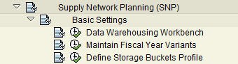

Selecting the Storage Buckets Profile brings up this screen below.

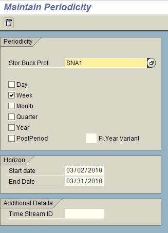
Here we are setting up the first profile, which will cover the next month. This will be set to weekly planning.

Here we have set up the following Storage Bucket Profile to cover the period following the initial month.

The first month could be called the procurement horizon (this is where purchase order recommendations are created). After that could be called the planning horizon (although technically, they are both within the planning horizon.) However, this description can be useful for many clients that find the term “frozen period” confusing.

This allows the data to be saved in a fixed number of days at the beginning of the planning horizon and after that in a larger bucket.

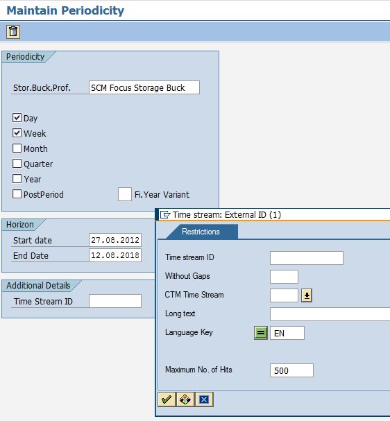
Selecting the Storage Buckets Profile brings up the screen on the following page, which allows the data to be saved in a fixed number of days at the beginning of the planning horizon and after that in a larger bucket.

How is the Storage Bucket Profile Assigned to the Planning Book?

The Storage Bucket Profile is assigned to the Planning Book through its assignment to the Planning Area. It is on the Info tab of the Planning Area.

The Planning Bucket Profile

As the names imply, the Planning Bucket Profile controls how the application displays the planning book’s data, and the Storage Bucket Profile controls how the application stores the planning data.

The Planning Bucket Profile defines how the data is planned and displayed in the planning books. The Planning Bucket Profile After the Storage Bucket Profile has been determined. The next logical step is to configure the Planning Bucket Profile, the purpose being to define the different sections of the horizon by making entries in the columns and the display periods.

Defining the Future Planning Horizon

The Planning Bucket Profile contains the periods or a subset of the periods you defined in the Storage Bucket Profile. Do not include a period in the Planning Bucket Profile that is not in the Storage Bucket Profile. These configuration steps define the future planning horizon and past horizon by entering them in a planning book—the duration for the future planning horizon and the past horizon. The future horizon starts with the smallest time bucket. The planning book must know how far in the past and how far into the future to look and to process information. Before we adjust the planning horizons, it is good to document the settings externally in a spreadsheet. By doing so, I can copy spreadsheets from previous clients and compare and contrast different configurations and timing settings.

So if we begin with the basics (i.e., what we want the Planning Bucket Profile to be), we can migrate this to SAP’s information input requirements. At the top of the next screenshot, I have placed what the Planning Bucket Profile should be in what could be called “plain English.”

After the Storage Bucket Profile has been determined, the next logical configuration step is the Planning Bucket Profile.

We go and select the Planning Buckets Profile item from SPRO.

When inside, we can choose any of the previously created ones, create our own…

SAP on the Planning Bucket Profiles

SAP has the following to say on Planning Bucket Profiles.

The first row defines the entire length of the time horizon. The following rows define the different sections of the horizon. You make entries in the columns Number (of periods) and Display periodicity. The content of the other columns is displayed automatically when you press Enter. To see exactly which buckets will be displayed, choose Period list. A planning buckets profile contains the periodicities or a subset of the periodicities that you defined in the storage buckets profile. In a planning buckets profile, do not include a periodicity that is not in the storage buckets profile. Having created planning bucket profiles, you use them to define the future planning horizon and the past horizon by entering them in a planning book: one for the future planning horizon and one for the past horizon. The system displays the horizons in interactive demand and supply planning by starting with the smallest time bucket and finishing with the largest time bucket. The future horizon starts with the smallest time bucket, on the planning horizon start date, and works forwards, finishing with the largest time bucket. The past horizon starts with the smallest time bucket the day before the start of the future horizon and works backwards, finishing with the largest time bucket. – SAP Help

In fact, it is not necessary to use a single periodicity. Multiple periodicities can be used to create a Time Bucket Profile, and thus what can be shown in the Planning Book.

The Configuration Area

I find this configuration area quite confusing. However, the book “Sales and Inventory Planning with SAP APO” has another excellent description of this screen’s logic.

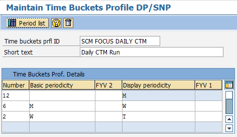
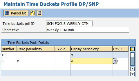
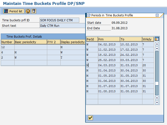
The time horizon comprises two years in the example shown. Of these two years, the first six months are shown in weeks. The first four weeks of the first month are shown in days. As we can see, the remaining 18 months are shown in months. The first line defines the entire length of the time horizon. The following lines define the various sections of the horizon. (emphasis added) You make entries in the columns Number and Display periodicity. The content of the other columns is displayed automatically as soon as you press Enter.

There is a quality check on this configuration object; this is described below:

If you want to see precisely what periods are displayed, click on the Period list button (see Figure 3.13).

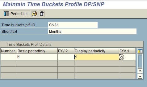
So the configuration is counterintuitive, but the thought process should be as if you are moving from less detailed to more detailed. So for a one-year planning horizon shown in months, it would be the following:

Year in Month

If you want the first six months to appear as weeks, then the following would be added.

Weeks then Months

A frequent request I hear is the ability to show closer planning periods in weekly planning buckets and monthly planning buckets after this.

The Way to See the Data

This is how most companies like to see their data, and it would also reduce the computation performed by SCM (i.e., not having to calculate weekly buckets out for the entire horizon. Creating a telescoping Time Bucket Profile is a frequent request for projects, and its configuration is counterintuitive. To find out how to create one see this article.

The next step is to convert the “plain English” version of what we want into the SAP Planning Bucket Profile setting. The first-row defines the entire length of the time horizon. The following rows define the different sections of the horizon. You make entries in the columns Number (of periods) and Display periodicity (or period types). The content of the other columns is displayed automatically when you press Enter. To see exactly which buckets will be displayed, choose Period list. A Planning Buckets Profile contains the periodicities or a subset of the periodicities that you defined in the Storage Buckets Profile. In a Planning Buckets Profile, do not include a periodicity that is not in the Storage Buckets Profile. Use the Planning Bucket Profiles that you created to define the future planning horizon and the past horizon by entering them in a planning book: one for the future planning horizon and one for the past horizon. The system displays the horizons in interactive demand and supply planning, starting with the smallest time bucket and finishing with the largest time bucket. The future horizon starts with the smallest time bucket on the planning horizon start date, and works forward, finishing with the largest time bucket. The past horizon starts with the smallest time bucket the day before the start of the future horizon and works backward, finishing with the largest time bucket. – SAP Help

Periodicities

It is not necessary to use a single periodicity (period type). Multiple periodicities can be used to create a Time Bucket Profile and can be shown in the Planning Book. The book Sales and Inventory Planning with SAP APO has an excellent description of this screen’s logic. The time horizon comprises two years in the example shown. Of these two years, the first six months are shown in weeks. The first four weeks of the first month are shown in days. As we can see, the remaining eighteen months are shown in months. The first line defines the entire length of the time horizon.

The following lines define the various sections of the horizon. You make entries in the columns Number and Display periodicity. The content of the other columns is displayed automatically as soon as you press Enter. To match our Planning Bucket Profile spreadsheet on the previous page, we would create the following entries in APO. Planning Bucket Profiles can be created with the same periodicity or with mixed periodicities.

When Periodicities are Mixed

When periodicities or period types are mixed (days, weeks, months, years), the vast majority of cases create a “telescoping” planning book. A telescoping planning book is used so that planners see small planning buckets close to the present day and successively larger planning buckets as the planning horizon reach out into the future. This is the preferred way for planners to see a planning book. Note that this has nothing to do with the Storage Bucket Profile, except that the Storage Bucket Profile must be as small as the smallest planning bucket used in the Planning Bucket Profile. To continue our example, we have decided upon the following telescoping planning bucket profiles.

One will begin with days, and the second for the MPS (master production schedule) will begin with weeks.

If you want to see precisely what periods are displayed, click on the Period list button.

While the configuration is counterintuitive, think of the process as moving from less detail to more detail.

I hear from clients that a frequent request is to show planning periods that will happen shortly in weekly planning buckets, with monthly planning buckets after this time period. Most companies would like to see their data in this manner, and doing so would reduce the computation performed by SCM (i.e., not having to calculate weekly buckets out for the entire horizon). The creation of a telescoping Time Bucket Profile is a frequent request for projects.

Initializing Planning Area

Planning Areas are the central data structure for both DP and SNP, and they hold the key figures used in many places but are shown prominently in the various DP and SNP Planning Books. Similar to the Storage Bucket and Planning Bucket Profiles, the Planning Areas must be initialized for both DP and SNP, and this transaction has a “from date” and “to date” as is described below:

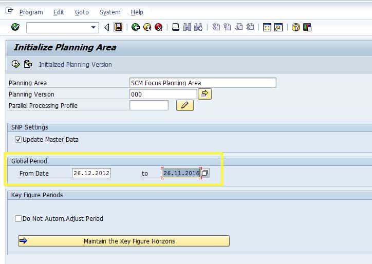
When using CTM, these settings interact with the CTM Time Stream (also known as the CTM Planning Calendar). Interestingly, this works in the exact opposite direction with the closer periods at the top. This configuration is much more logical than the Planning Bucket Profile.

This is shown in the screenshot below:

How these timing configurations interact is shown in the graphic below: Storage and Planning Bucket Profiles

Go to top

Conclusion

This post demonstrates that the periodicity the data is stored in is not necessarily the same displayed. To find out more about the logic for setting the Time Bucket Profile, see the following article.

References

https://www.sap-press.de/katalog/buecher/htmlleseproben/gp/htmlprobID-146